Création d’une digue synthétique

Import des modules

# import _add_path # for debugging purposes only - must be removed in production

import pandas as pd

from wolfhece import is_enough
if not is_enough('2.2.35'):
    raise ImportError("This code requires wolfhece version 2.2.35 or higher. -- try pip install wolfhece --upgrade")

from wolfhece.pydike import SyntheticDike
from wolfhece.PyVertexvectors import vector
from wolfhece.wolf_array import WolfArray, header_wolf
from wolfhece.analyze_poly import Slope_analysis, Array_analysis_onepolygon

import numpy as np

from unittest import TestCase, main
import matplotlib.pyplot as plt

Création d’une digue sur base d’une trace, de pentes et d’altitudes min et max

L’amont est défini comme étant à droite de la trace. L’aval est la gauche de la trace.

Une digue a les propriétés suivantes :

• une largeur amont (largeur en tête de digue)

• une largeur aval

• une pente amont

• une pente aval

La trace n’est donc pas située au milieu de la digue, sauf si les deux largeurs sont identiques.

dike = SyntheticDike() # Create a SyntheticDike object

trace = vector('dike_trace') # Create a vector for the dike trace

trace.add_vertices_from_array(np.asarray([[0.,0.,0.],
                                          [10,10,0.]])) # Add vertices to the trace vector

# Define the slopes and widths for the dike
width_up   = 0.0  # No width at the top of the dike
width_down = 0.0  # No width at the bottom of the dike
slope_up   = 2.0  # Slope of the dike - upstream side -- slope défined as dZ / dX
slope_down = 5.0

# Create the dike triangulation with zmin and zmax
zmin = 0.0  # Minimum z-coordinate for the dike
zmax = 10.0 # Maximum z-coordinate for the dike
ds = 1.0    # Distance between vertices in the dike trace

dike.create_from_slopes(trace,
                        slope_up, slope_down,
                        width_up, width_down,
                        zmin, zmax,
                        ds)

tri = dike.triangulation # Get the triangulation object from the dike
zones = dike.zones # Get the "Zones" instance from the dike triangulation

%matplotlib inline
# Plotting the triangulation in 3D
fig = plt.figure()
ax = fig.add_subplot(projection='3d')
tri.plot_matplotlib_3D(ax)
ax.set_aspect('equal')
fig.show()

# Plotting the dike trace and zones in 2D
fig, ax = plt.subplots()
zones.plot_matplotlib(ax)

trace.myprop.color = (255,0,0)
trace.myprop.width = 2.0
trace.plot_matplotlib(ax)

ax.set_aspect('equal')
plt.show()

C:\Users\pierre\AppData\Local\Temp\ipykernel_16156\370630881.py:34: UserWarning: FigureCanvasAgg is non-interactive, and thus cannot be shown
  fig.show()

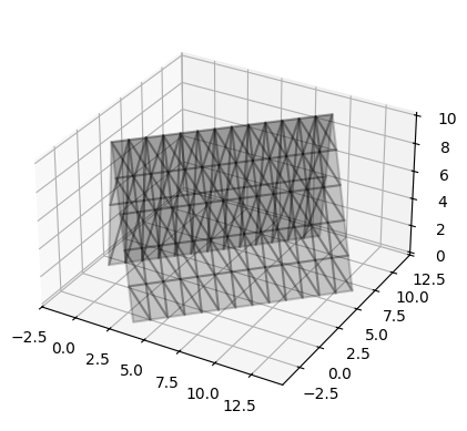
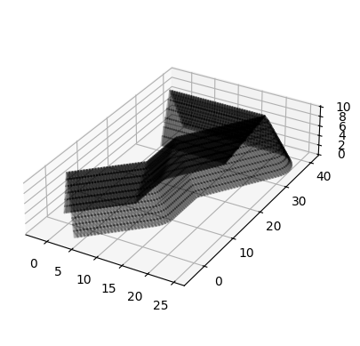
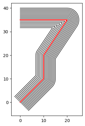
Création d’un digue sur base d’une forme de section

On définit ici:

• une trace

• une forme de section transversale de la digue

La routine “create_from_shape” va ensuite distribuer au mieux la forme selon la trace.

dike = SyntheticDike()

trace = vector('dike_trace')
shape = vector('dike_shape')

trace.add_vertices_from_array(np.asarray([[0.,0.,10.],
                                          [10,10,10.],
                                          [10,20,10.],
                                          [20,35,10.],
                                          [0,35,10.]]))
width_up = 0.0
width_down = 0.0
slope_up = 2.0
slope_down = 3.0

zmax = 10.0
zmin = 0.0

shape.add_vertices_from_array(np.asarray([[-(zmax - zmin) / slope_down, zmin],
                                            [0.,zmax],
                                            [(zmax-zmin) / slope_up,zmin]]))


ds = 0.5

dike.create_from_shape(trace, shape, ds)

tri = dike.triangulation
zones = dike.zones

%matplotlib inline
fig = plt.figure()
ax = fig.add_subplot(projection='3d')
tri.plot_matplotlib_3D(ax)
ax.set_aspect('equal')
fig.show()

# Plotting the dike trace and zones in 2D
fig, ax = plt.subplots()
zones.plot_matplotlib(ax)

trace.myprop.color = (255,0,0)
trace.myprop.width = 2.0
trace.plot_matplotlib(ax)

ax.set_aspect('equal')
plt.show()

C:\Users\pierre\AppData\Local\Temp\ipykernel_16156\993472420.py:36: UserWarning: FigureCanvasAgg is non-interactive, and thus cannot be shown
  fig.show()

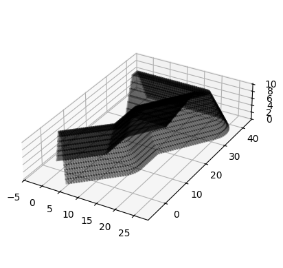
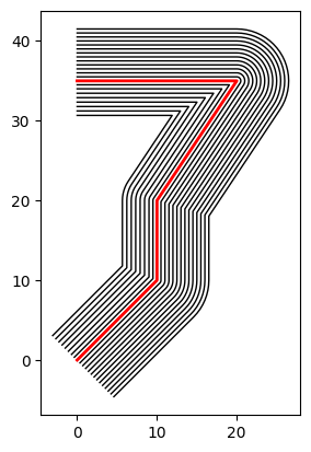
Même approche mais avec une largeur non-nulle en tête de digue

dike = SyntheticDike()

trace = vector('dike_trace')
shape = vector('dike_shape')

trace.add_vertices_from_array(np.asarray([[0.,0.,10.],
                                            [10,10,10.],
                                            [10,20,10.],
                                            [20,35,10.],
                                            [0,35,10.]])) # The trace has the same elevation at each vertex
width_up = 1.5
width_down = 1.0
slope_up = 2.0
slope_down = 3.0

zmax = 10.0
zmin = 0.0

shape.add_vertices_from_array(np.asarray([[-width_down -(zmax - zmin) / slope_down, zmin],
                                            [-width_down, zmax],
                                            [0.,zmax],
                                            [width_up, zmax],
                                            [width_up + (zmax-zmin) / slope_up,zmin]]))


ds = 0.5

dike.create_from_shape(trace, shape, ds)

tri = dike.triangulation
zones = dike.zones

%matplotlib inline
fig = plt.figure()
ax = fig.add_subplot(projection='3d')
tri.plot_matplotlib_3D(ax)
ax.set_aspect('equal')
fig.show()

# Plotting the dike trace and zones in 2D
fig, ax = plt.subplots()
zones.plot_matplotlib(ax)

trace.myprop.color = (255,0,0)
trace.myprop.width = 2.0
trace.plot_matplotlib(ax)

ax.set_aspect('equal')
plt.show()

C:\Users\pierre\AppData\Local\Temp\ipykernel_16156\3333825595.py:38: UserWarning: FigureCanvasAgg is non-interactive, and thus cannot be shown
  fig.show()

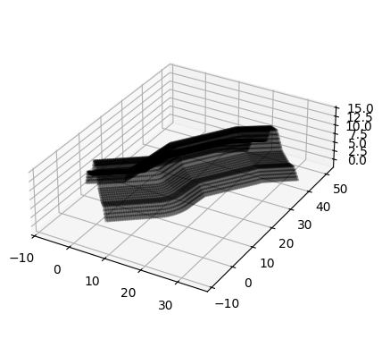
Interpolation sur une matrice de topographie

Dans cet exemple, la trace évolue en altimétrie.

La forme de la digue est toujours définie de façon relative, c’est-à-dire que la sommet de la digue sera positionné à l’altitude locale définie par la trace.

%matplotlib inline
#%matplotlib widget # Uncomment this line to use interactive widgets in Jupyter Notebook

dike = SyntheticDike()

trace = vector('dike_trace')
shape = vector('dike_shape')

trace.add_vertices_from_array(np.asarray([[0.,0.,15.],
                                            [10,10,14.],
                                            [10,20,13.],
                                            [20,35,13.],
                                            [25,45,10.],
                                            ])) # The elevation changes along the trace
width_up   = 1.5
width_down = 1.0
slope_up   = 2.0
slope_down = 3.0

zmax = 10.0
zmin = 5.0

shape.add_vertices_from_array(np.asarray([[-11., -2.],
                                            [-9., 2.5],
                                            [-7., 3.],
                                            [-width_down -(zmax - zmin) / slope_down, zmin],
                                            [-width_down, zmax],
                                            [0.,zmax],
                                            [width_up, zmax],
                                            [width_up + (zmax-zmin) / slope_up, zmin],
                                            [7., 3.],
                                            [9., 3.],
                                            [11., 0.]]))


ds = 0.5

dike.create_from_shape(trace, shape, ds)

tri = dike.triangulation
zones = dike.zones

fig = plt.figure()
ax = fig.add_subplot(projection='3d')
tri.plot_matplotlib_3D(ax)
ax.set_aspect('equal')
plt.show()

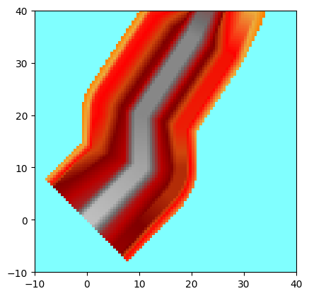
h = header_wolf()
h.set_origin(-10, -10)
h.set_resolution(0.5,0.5)
h.shape = (100, 100)

a = WolfArray(srcheader=h)

a.interpolate_on_triangulation(tri.pts, tri.tri, keep = 'above') # Interpolate the triangulation points onto the array
# The "keep" argument is set to 'above' to retain all values above the array.
# Other options for "keep" are 'all' or 'below'.
# If "all" is used, no filtering is performed and all values are kept.
# If "below" is used, only values below the array are retained.

fig, ax = a.plot_matplotlib()
plt.show()