Supported formats
Text files
Encoding convention
The text WOLF files use ascii-ANSI format with characters CR + LF (ASCII 13 + 10) at the end of each line.
Separator in-between values on the same line can be comma or space.
Boolean
Boolean must be written #TRUE# or #FALSE# (VB6 like format - uppercase).
Null value
All optional values can be defined as “0” or “-99999” (null value in WOLF) if not relevant.
JSON files
Some recent paremeters files use JSON format. The JSON format is a text format that is completely language independent but uses conventions that are familiar to programmers of the C-family of languages, including C, C++, C#, Java, JavaScript, Perl, Python, and many others.
Json is used by some WOLF Python classes (GPU, particles…) to serialize and deserialize objects.
Json files are not retrocompatible with the previous text files.
(multi)Polygon, (multi)Polylines
Vector files (.vec, .vecz)
Associated class Zones
A vector file is an ASCII text file with an extension “.vec” (2D coordinates) or “.vecz” (3D coordinates).
2D and 3D data cannot be mixed.
There are four types of components:
The content of the file is a concatenation of components, beginning with optional translation coordinates:
Translation coordinates to real world (float, float) (optional)
Number of zones (integer): nb_zones
- For each zone:
Name-ID (character 255 max.)
Number of vectors (integer): nb_vect
- For each vector:
Name-ID (character 255 max.)
Number of vertices (integer): nb_coord
Enumeration of the x-y or x-y-z coordinates (float, float (float)) - one pair/triplet of coordinates
Vector properties
…
Example :
0.000000 0.000000
1
zone
2
vector_1
4
1.000000 1.000000
1.000000 4.000000
4.000000 4.000000
4.000000 1.000000
0, 1, 0,#TRUE#,#FALSE#,#FALSE#,#FALSE#, 0,#FALSE#
"...", 5, 0.000000, 0.000000,#FALSE#,#FALSE#,"arial", 10, 0,#FALSE#
#TRUE#
vector_2
4
2.500000 1.000000
3.500000 2.000000
2.000000 3.500000
1.000000 2.500000
0, 1, 0,#TRUE#,#FALSE#,#FALSE#,#FALSE#, 0,#FALSE#
"...", 5, 0.000000, 0.000000,#FALSE#,#FALSE#,"arial", 10, 0,#FALSE#
#TRUE#
Extra files ‘.vec.extra’
An extra properties file, ASCII text, can be read/write for each .vec/vecz file.
These properties are related to the legend, picture attached to the vector, etc.
This file is only compatible with the Python version of WOLF.
Shapefiles
Shapefiles (.shp, .shx, .dbf) are a popular geospatial vector data format for geographic information system (GIS) software. The shapefile format can spatially describe vector features: points, lines, and polygons.
The format is composed of several files:
.shp: the main file containing the geometry
.shx: the index file
.dbf: the attribute file
You can import shapefiles in WOLF. The shapefile is converted to a Zones class.
Every polygon or polyline is converted to a Zone class and a vector instance. If some parts are detected in the polygon, multiple vectors are created, one for each part.
Shapefiles are used mainly for the geometry, not the attributes.
Read/Write operations are delegatted to Geopandas library.
Internal conversion use Shapely library. Indeed, Wolf can convert a zone or vector instance to a Shapely object and vice versa.
DXF files
DXF files are date exchange files. They are used to exchange data between different CAD programs. There is a limited support of DXF files in WOLF. The support is limited to the reading of the 2D polylines and polygons.
DWG files are the native format of AutoCAD. They are not supported by WOLF.
So, if you want to use a DWG file in WOLF, you have to convert it to a DXF file with a CAD program.
Arrays
Binary files (.bin)
.bin files are binary files containing arrays of values.
A header file must be provided to read the binary file. The header file is an ASCII text file with an extension “.bin.txt”.
It contains the following information:
NbX : Number of cells in the X direction (integer)
NbY : Number of cells in the Y direction (integer)
OrigX : X coordinate of the lower-left corner in local system (float)
OrigY : Y coordinate of the lower-left corner in local system (float)
DX : size of the cell in the X direction (float)
DY : size of the cell in the Y direction (float)
TypeEnregistrement : integer value coding the type of the data (1 = float32, 2 = float64, 6 = integer32…)
TranslX : Translation in the X direction to be in real world system (float)
TranslY : Translation in the Y direction to be in real world system (float)
Coordinates of the cell center are calculated as follows:
Example:
NbX :       68076
NbY :       15088
OrigX :     0
OrigY :     0
DX :        0.5
DY :        0.5
TypeEnregistrement :        1
TranslX :   237800.0
TranslY :   139850.0
The binary part of the file (.bin) contains the values of the array.
The shape of the array is [NbX, NbY]. So, the first index varies as the X direction and the second index is the Y direction.
The file size can be calculated as follows:
Note
For reminder, float32 is 4 bytes, float64 is 8 bytes, integer32 is 4 bytes.
In the real world, the first element, [0,0] in Python, corresponds to the lower-left element of the array. However, from a numerical/informatics perspective, the first element [0,0] is the upper-left element of the matrix.
The values are stored in column-major order - Fortran convention. The most rapid varying index is the first one, i.
Attention
The WOLF convention is different from the matrix convcention where the first index is the line and the second index is the column.
One is the transpose of the other.
Wolf format can not store multiple bands in a single file.
Geotiff files (.tif)
Geotiff files are raster files with georeferencing information. Date can be stored in different formats (float32, float64, integer32…) and compressed using LZW algorithm.
Wolf can read and write Geotiff files, by using GDAL/Geopandas.
A Geotiff file can contain multiple bands. Each band is a 2D array of values.
Wolf can write 2D results in a multiple bands Geotiff file.
Attention
The convention is different from the Wolf binary files. To read Geotiff files in wolf_array, the code will flip/transpose axis after reading binary data.
Float ESRI (.flt)
Float ESRI (.flt) files are raster files with georeferencing information. Data are stored in float32 format.
Attention
The convention is different from the Wolf binary files. To read flt files in wolf_array, the code will flip/transpose axis after reading binary data.
Numpy files (.npy)
Numpy files (.npy) are binary files containing one array of values.
Wolf can read and write .npy files.
Attention
By default, npy file does not contain georeferencing information. The user must provide a header file to read the file in the correct way.
Numpy files (.npz)
Numpy files (.npz) are binary files containing multiple arrays of values.
Wolf can read and write .npz files.
Attention
By default, npz file does not contain georeferencing information. The user must provide geographic information in a ‘header’ array inside the npz.
This array must contain the 6 following information: (origx, origy, dx, dy, nbx, nby)
If the header is not provided, the used values are (0., 0., 1., 1., shape[0], shape[1])
Parameters files
Parameters (.param, .param.default)
See Pyparams.Wolf_Param for more information on how this file is managed.
A parameter file is an ASCII text file with an extension “.param” or “.txt”.
The main purpose of the parameter file is to provide the user with a simple way to modify the input data of the simulation. Another purpose is to facilitate the exchange of values between Python and Fortran codes.
Parameters can be organized into groups. A group is identified by a name-ID (case insensitive) followed by a colon “:”.
Each parameter is defined on the same line, separated by a tab:
name
value
comment (optional)
Multiple occurrences of the same parameter name can occur in different groups. In one group, only once occurrence of the name is allowed.
Line starting with “%” or blank line is considered as a comment. Comment can be used to describe the parameter – see Json.
Example :
Time :
Maximum iteration   10      Number of iterations (integer)
Maximum time        1.00000000000000000000E+01      Time of simulation (double, seconds)
Round Time  0.00000000000000000000E+00      Forced time interval (double)
Local time_stepping 0       Local time stepping - 0 = .false., 1 = .true. (integer)
Start Time  0.00000000000000000000E+00      Starting time (double)
Results :
Write frequency     1.00000000000000000000E+00      Writing interval (integer or double)
Write type  1       Testing type - iterations = 1, time = 2 (integer)
Spatial scheme :
Reconstruction      1       Reconstruction method - constant = 1, linear = 2 (integer)
Temporal scheme :
RK model    2       Runge-Kutta scheme - 1, 2 or 3 (integer) - (n-1) coefficients to provide
RK Coeff (2)        5.00000000000000000000E-01      Second coefficient (double)
Courant Number      2.50000000000000000000E-01      Limitation of the time step through the Courant number (double)
Limitations :
Maximum Froude      2.00000000000000000000E+01      Limitation of the results through the Froude number (double
Source Terms :
Friction Law        3       Friction law - Bazin = 1, Colebrook = 2, Manning = 3, Barr-Bathurst = 4
Verbosity :
Code Verbosity      0       Verbosity of the computation - 1 = .true. , 0 = .false. (integer)
Type of values
The type of the value is defined by the Fortran code in the comment attached to the value. The type can be integer, double, float, logical, character, file, directory…
In the Python code, the type is not checked. The value is converted to the type defined in the comment.
Default parameters
A default parameters file is an ASCII text file with an extension “.param.default”, “.txt.default”.
The default parameters file is normally written by the Fortran code and contains the first initialized values.
During the initialization phase, first values are chosen by default. Then, the “.param” file is read and only the specified values are overwritten.
In this way, the “.param” file can only contain the modified values.
If the user decides to copy-paste the default file, rename it and modify some values, the result will be the same but the readability (in text editor like Notepad++) is lower.
Json
Some recent parameter files (GPU Simple Simulation…) use the JSON format.
In a “.param” file, a line beginning with “%json” can be used to associate text with an integer value. This line is used by Wolf to display the values as a listbox in the GUI instead of a numerical value. The key-value pairs are provided as a Python dictionary under the “Values” key.
A more detailed comment can be added to the line to describe the parameter. This comment will be displayed in the multiline textbox at the bottom of the parameter GUI.
Example:
%json{"Values":{Manning:1, Strickler:2, Barr-Bathurst:3}, "Full_Comment":Choix de la loi de frottement\nValeurs possibles : Manning, Strickler, Barr-Bathurst}
Point cloud
Point cloud files can be imported, optionally accompanied by attributes.
These data can be in the form of XYZ files, shapefiles, or LAS/LAZ files.
XYZ files
In the case of XYZ files, additional columns can be added to define attributes. The first line defines the column names.
Cloud points can be triangulated (Delaunay) to create a mesh.
Lidar files
Lidar data can be imported in the form of LAS or LAZ files. The laspy library is used for this purpose.
Although LAZ files are stored in binary and compressed form, specific classes have been coded to improve data accessibility. In particular, the data is redistributed on a small spatial scale (e.g. 50 m x 50 m) and stored in the form of Numpy tables, so that loading only the data required for display at different zoom levels.
Lidar data can be viewed in the WOLF graphical interface via a separate viewer based on the pptk library. The viewer can be used to display large point clouds (more than 50 million) in real time.
The colours used can either be based on the classification of the points (ground, above ground, bridge, etc.) via a conversion table, or on the RGB colours of an aerial image for the same spatial coverage (automatic recovery via Walonmap webservices, for example).
Derived types
The previous types serve as a basis for defining more complex types.
Cross sections
Cross sections are considered as a series of 3D polylines. Each section has its representation in the real world (X, Y, Z) but also in local axes (S, Z), oriented positively from the left bank to the right bank according to the section trace.
Reference points can be associated:
Bottom of the minor bed
Left bank
Right bank
Cross sections can be spatially interpolated on a grid after 3D triangulation.
Triangulation
Triangulation is a data structure that allows representing 3D surfaces from 3D points and the segments connecting them.
The internal storage mode involves storing the 3D points in a vector and defining the segments based on position indices.
Triangulation can be stored in a binary file “.tri” (similar to the STL format) or in the form of “.glb/.gltf” files for 3D visualization/sculpting in Blender.
Tiles
Tiles are a combination of spatial footprint, in the form of polygons, and associated data.
The associated data can be:
arrays/matrices (Lidar data, …)
images (land surveys, …)
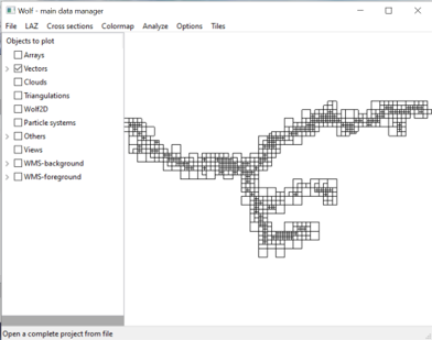
Exemple of tiles for Lidar 2023 - Vesdre (Belgium) dataset.
Note
Others types can be added/described in the future.