Drowning
The drowning model is developped in the thesis of Clément Delhez (2025).
Note
All the details on its content can be found in his thesis or in the following scientific publications.
Force coefficients for modelling the drift of a victim of river drowning
New articles are in preparation and will be available soon.
The drowning model is a Lagrangian one, performing Monte Carlo runs using a second-order Runge-Kutta (RK22) time integration scheme with a variable time step defined by a CFL and minimum and maximum time steps. Everything in the model is parallelised and can be easily divided in multiprocesses to speed up the simulation. It solves the equations of motion along with Newton’s second law. The forces taken into account include: drag, lift, lateral lift, the body’s weight, its buoyant force, Coulomb bottom friction, and added mass forces. The model incorporates a decomposition process based on an intrinsic procedure, allowing the body’s volume to evolve over time as a function of water temperature, depth, and the body’s characteristics. The presented model starts from a fluid velocity averaged over depth and infers a position-dependent velocity, which varies according to the body’s location within the mesh cell, its vertical position, and the preceding and following time steps of the velocity field simulation (via linear temporal interpolation). It also includes a stochastic component in the horizontal flow velocity. The collision model is elastic and only reduces the body’s velocity in the direction perpendicular to the wall.
In the proposed version, the model uses WOLF GPU 2D results as a flow field. A first order of idea of computation time is 1 hour of computation time by drowning day with a computer having 16 chores and 13 parallel processes, 10.000 Monte Carlo runs and default CFL number and a_1.
Data
As mentionned, this version of the model requires WOLF GPU 2 results to work. Make sure, to have your flow simulation ready and covering more than the drowning period (an extra hour of simulation is recommended). All the other data are recommended but not mandatory. The model will work without them but the results will be less accurate.
Initialisation/Create a drowning
Start wolf with the command.
wolf
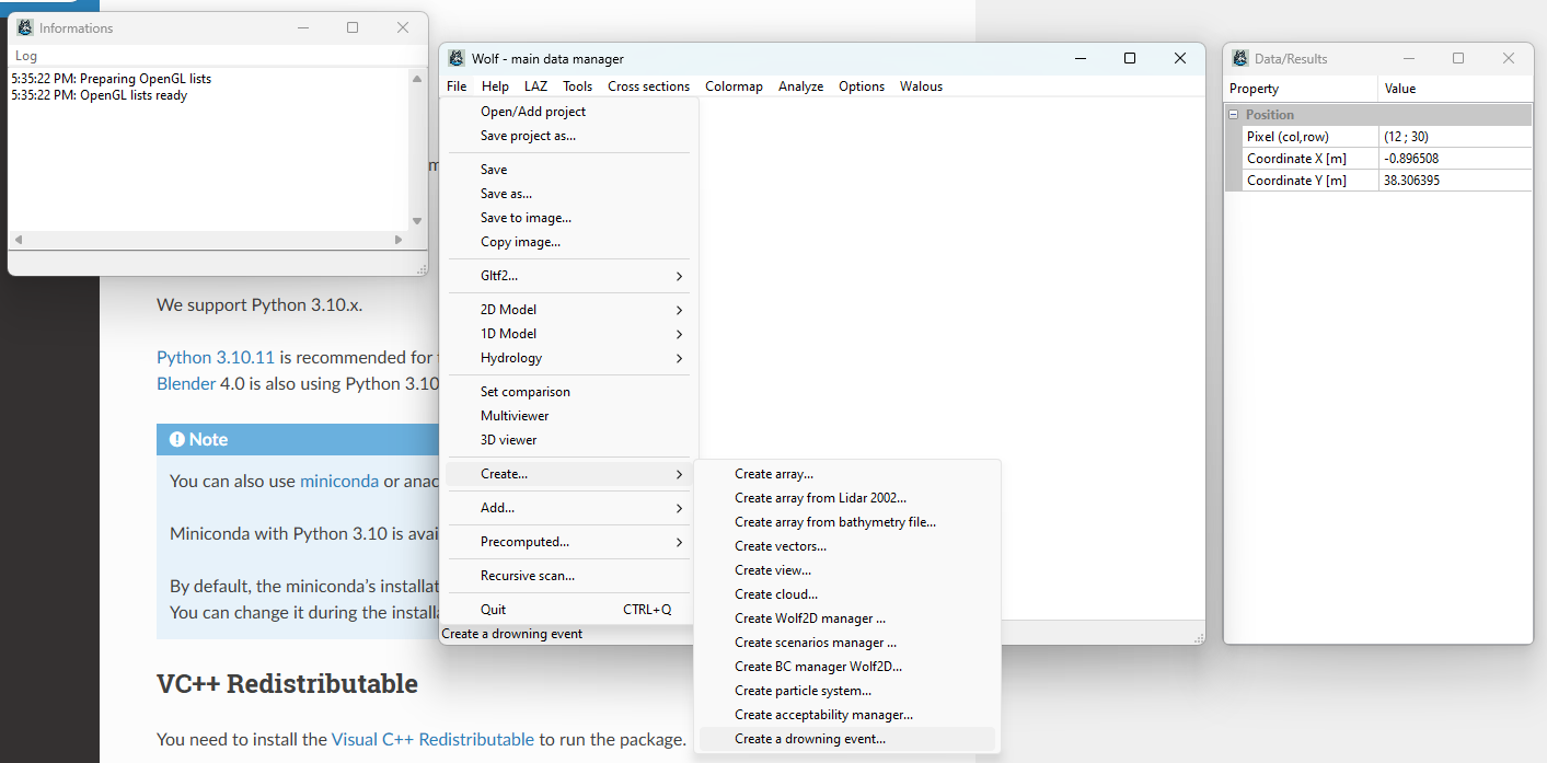
From the opened graphic interface, create a drowning by selecting Create a drowning….
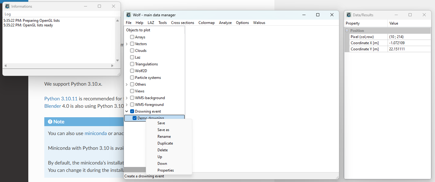
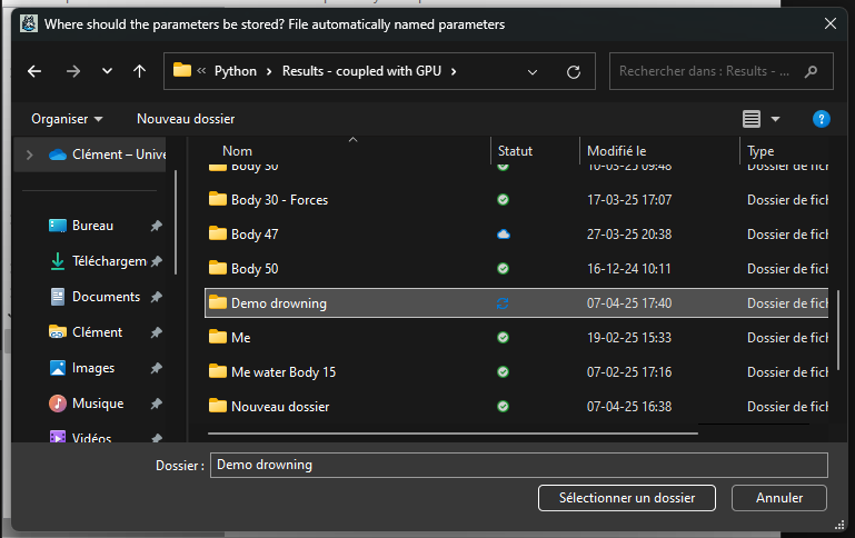
A drowning object is created. You can already Save you drowning into a specific folder used for this drowning simulation. Left click on the drowning object and select Save.
Note
The save step is not mandatory at this point but is recommend as it will be mandatory for the execution file creation.
Parameters/Propreties of the drowning
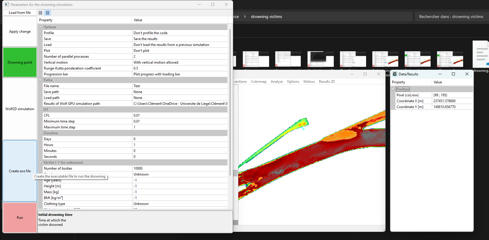
You can now edit the propreties of your drowning. Left click on the drowning object and select Propreties. A window opens with all the editable parameters. The window is subdivided in 3 parts: - Interactive buttons. - Active parameters. - Default parameters.
Active parameters
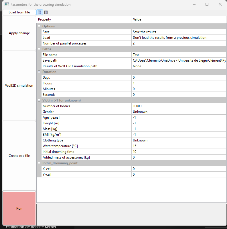
The window of active parameters is the window directly open when you select Propreties. Here is a list of each parameter and its description:
Options
Save : Choose if you want to save the drowning or not. (Save the results:1, Don’t save:0)
Load : Choose if you want to load a previous drowning or not. (Load:1, Don’t load:0)
Number of parallel process: Number of parallel process to use for the simulation. Define the number of parallel process to use for the simulation, with a minimum to 1. Check the number of chores of your computer before selecting it. With a computer having 16 chores, choosing 13 parallel processes allows the computer to work normally and the model to be efficient.
Paths
File name : Name of the drowning.
Save path : Path to the folder where everything will be saved. If you already saved your drowning object, the saving path will automatically update.
Results of Wolf GPU simulation path : Path to the folder where the WOLF GPU simulation is stored. This path is mandatory and is automatically updated after selecting the button Wolf2D simulation.
Duration
Days : Number of days of the simulation. Can only be an integer.
Hours : Number of hours of the simulation. Can only be an integer.
Minutes : Number of minutes of the simulation. Can only be an integer.
Seconds : Number of seconds of the simulation. Can only be an integer.
Victim (-1 for unknown)
Number of bodies : Number of runs in the Monte Carlo simulation. Affects a lot the simulation time. The more runs, the more accurate the results but the longer the simulation. Must be bigger than your number of parallel processes.
Gender : Gender of the victim. If unknown, set to -1.
Age : Age of the victim in years (integer). If unknown, set it to -1.
Height : Height of the victim in m (float). If unknown, set it to -1.
Mass : Mass of the victim in kg (float). If unknown, set it to -1.
BMI : Body Mass Index of the victim (float). If unknown, set it to -1. Is used only if the mass of the victim is unknown. If the body mass is known, the BMI is calculated from the mass and height of the victim.
Clothing type : Type of clothing of the victim. If unknown, set it to -1. The clothing type is used to calculate the drag coefficient and the volume of the body.
Water temperature : Average water temperature during the drowning in °C (float). If unknown, set it to -1. The water temperature is used to calculate the decomposition of the body (and so, its volume).
Initial drowning time : Hour at which the victim drowned. If unknown, set it to an arbitrary value. Example: if someone drowned at 10:00, set it to 10.
Added mass of accessories : Added mass of accessories in kg (float). If none, set it to 0. An added mass of accessory can be a backpack of 5 kg (-> 5 kg) or a life jacket reducing the mass of 2 kg (-> -2 kg, considreing that the accessories only have an effect on the mass and not the volume).
Initial_drowning_point
X-cell : Index of the cell in the x direction where the victim drowned. Is automatically changed during the procedure of selection a drowning point.
Y-cell : Index of the cell in the y direction where the victim drowned. Is automatically changed during the procedure of selection a drowning point.
Default parameters
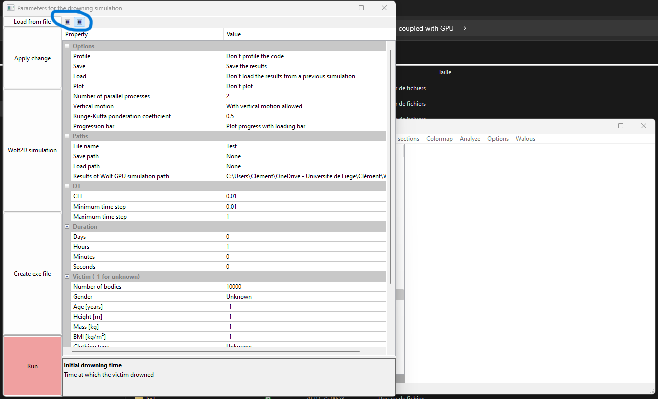
The window of defaut parameters is the window openend when you select the right box in the surrounded area. You can change the value of a default paramter by double left clicking on its name. It will go to the active window and you can change its value as an active parameter. Here is a list of each default parameter and its description:
Options
Profile : Choose if you want to profile your code or not (have a list of the computation time taken by each function). (Profile:1, Don’t profile:0)
Plot : Choose if you want to plot the results directly at the end of the simulation or not. (Plot:1, Don’t plot:0)
Vertical motion : Choose if you want to take into account the vertical motion of the body or not. (Vertical motion:1, Pure horizontal motion:0)
Runge-Kutta ponderation coefficient : Ponderation coefficient of the Runge-Kutta method. The default value is 0.5. The value must be between 0 and 1. A value of 0.5 is the default value of the RK22 method.
Progression bar : Choose if you want to see the progression bar or an progression image. (Progression bar:1, Progression image:0)
Paths
Load path : Path to the folder where the base drowning is stored. Considered only if parameter Load is activated.
DT
CFL number : CFL number used for the simulation. The value must be in ]0;1].
Minimum time step : Minimum time step used for the simulation in seconds.
Maximum time step : Maximum time step used for the simulation in seconds.
Apply changes to parameters
Once you have modified the relevant parameters, select Apply change.
Note
You can also select Load from file to load an existing drowning from a file parameter.param.
Choose your reference WOLD 2D GPU simulation
Select the button Wolf2D simulation to select the WOLF 2D GPU simulation you want to use for the drowning simulation. A window opens in which you have to choose for a folder containing a WOLF simulation.
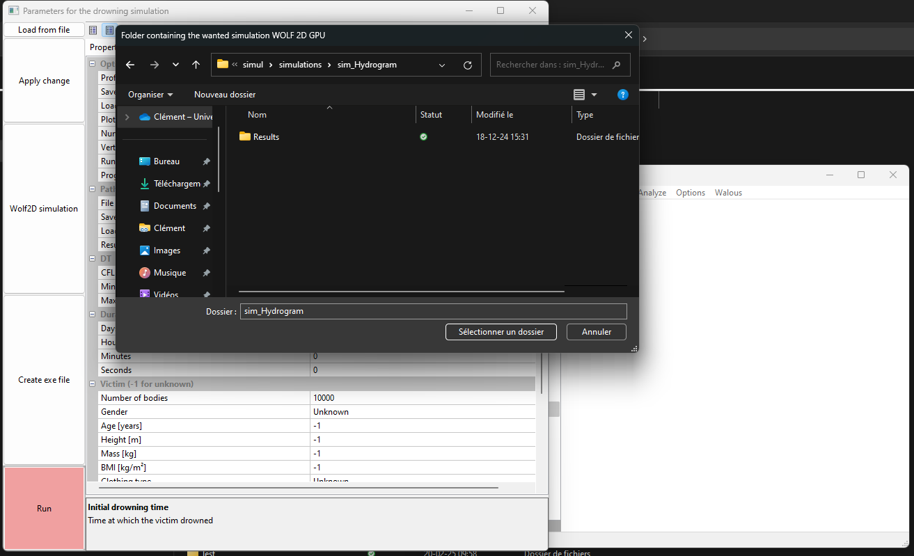
When the folder is selected, the simulation is automatically loaded and the path is updated in the Results of Wolf GPU simulation path field.
You can then zoom on the drowning area and select the drowning point (exemple: by choosing a node by node selection with the shortcut n and then a right click on the appropriate cell).
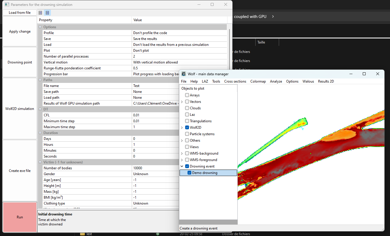
Once your drowning point is selected, select the button Drowning point to update the drowning point in the parameters. If everything is ok, the Drowning point button becomes green. The window won’t update automatically but the values of the drowning point are updated in the parameters. You can check it by closing the window and selecting Propreties again. The X-cell and Y-cell values are updated. Be carefull, if you have selected less or more than one drowning point, you will have an error message and need to select only one to continue.
Save your final parameters
Don’t forget to save your parameters by selecting Save in the drowning object. You can also select Save as… to save your parameters in another folder or with another name if wanted.
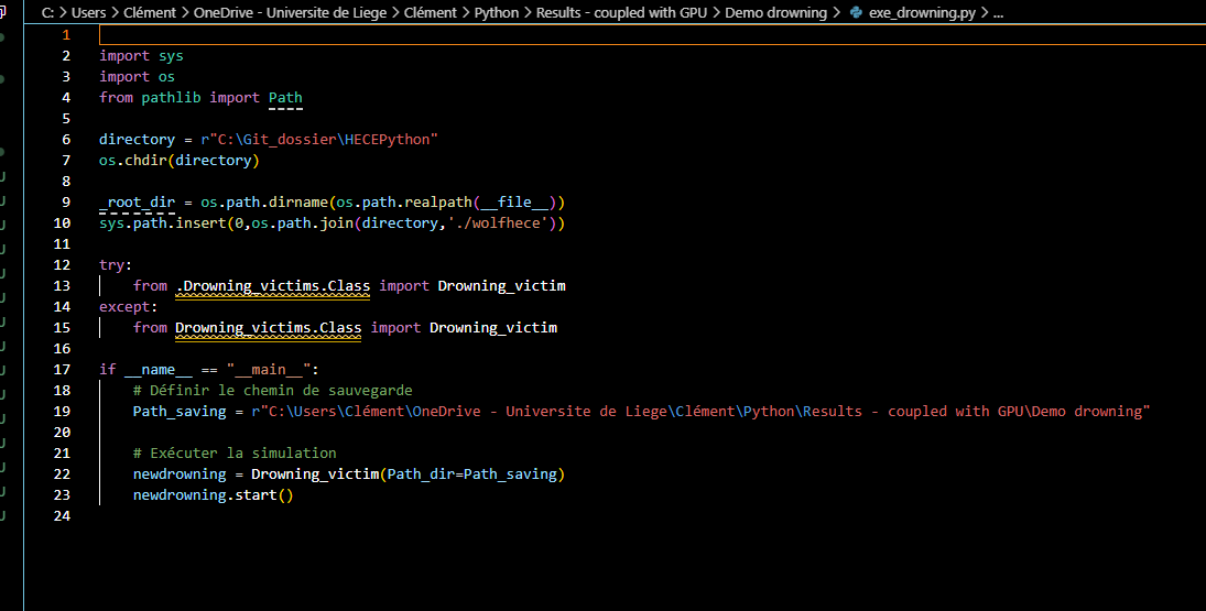
Create an executable file
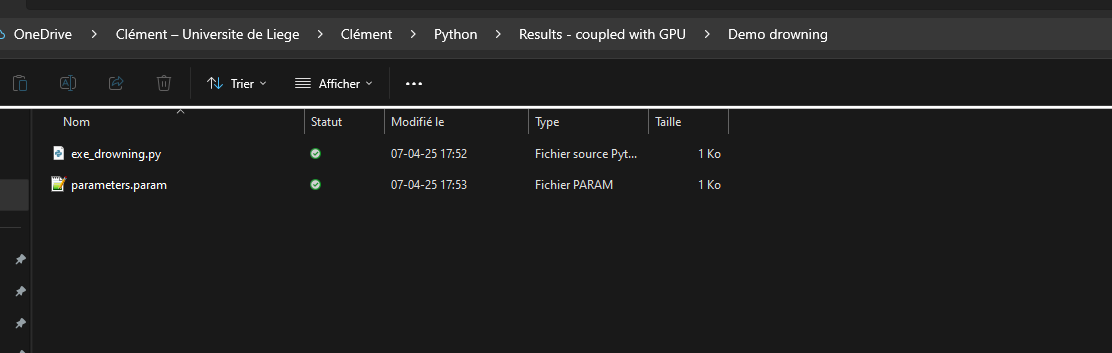
Once you have selected a storing directory, you can create an executable file by selecting the button Create exe file. The purpose of this file is to generate an autonomous execution file for the simulation. As mentionned earlier, a drowning simulation is very time consuming (as drownings can last for days and weeks). It is so recommended to start a simulation by running the exe_file in a different terminal to be able to keep working in the current one.
Once you have created your exe_file, you see a message in your terminal indicating where it is stored and you can see it in your reference folder.
Start your simulation
At this stage, you can start your simulation either by clicking on the button Run, knowing that it will block your current terminal with the simulation; or by running the exe_file in a different terminal.
Both methods are equivalent for the drowning simulation.
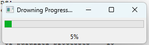
Once the simulation is started, the model enters to the initialisation procedure (for a few seconds) and then, when entering the main loop, you will see your progression bar (or image) appearing. The progression bar considers the evolution of the slowest process.
Results
When the simulation is over, a file Results.npz is created in the folder you selected for the simulation. This file contains all the results of the simulation. You can open it with python and numpy. The file contains 6 arrays: - Path_save : Path to the folder where the results are saved. - Pos_b : An array of shape (n_b,3,n_t) with n_b the number of Monte Carlo runs, 3 the coordinates (x,y,z) and n_t the number of time steps. The array contains the 3D position of the body at each time step. - U_b : An array of shape (n_b,3,n_t) with n_b the number of Monte Carlo runs, 3 the coordinates (u,v,w) and n_t the number of time steps. The array contains the 3D velocity of the body at each time step. - Human : A DataFrame pandas containing all the simulated bodies and their characteristics (one body per line) - Z_param : A DataFrame pandas containing the vertical parameters of all the simulated bodies (one body per line). - wanted_time : An array of shape (n_t) with n_t the number of time steps. The array contains the time of each save in seconds. Example: if wanted_time[1] = 1, then Pos_b[0,0,1] is the x coordinate of the body 0 at time 1 second. - time_b : An array of shape (n_b,n_t) with n_b the number of Monte Carlo runs and n_t the number of time steps. The array contains the time of each body at each time step.
If you choose a simulation with only one process, you also have a folder named Results filed with results.npz file for each saved step.
Read results through the graphic interface/Add a drowning…
Open the file menu and go to Add a drowning result…. Choose the folder containing your drowning files (give the folder that you created when saving your drowning, as in the last figure juste before the section Parameters/Propreties of the drowning). A drowning object is created but nothing happens.
Plots
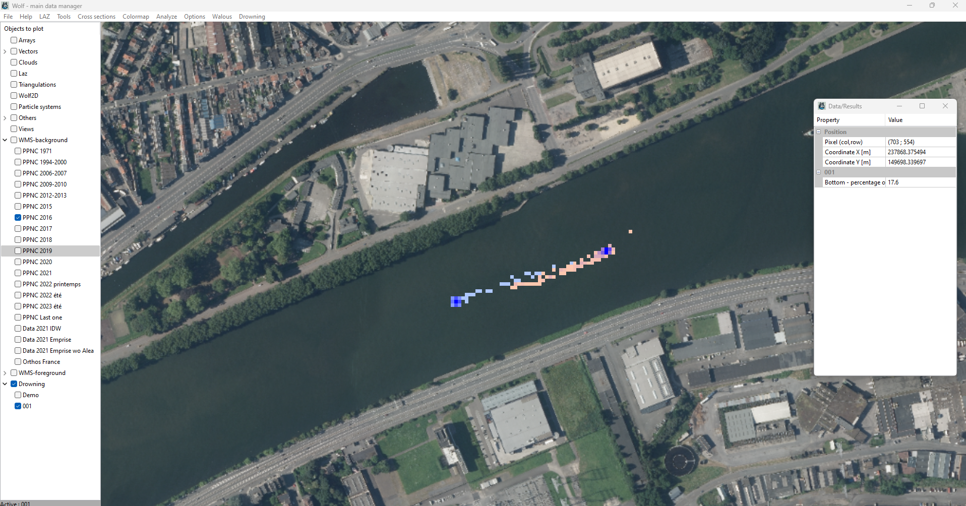
Keep in mind that in this section, the blue color is always associated to bodies on the bottom and the red color is always associated to the surface.
For a drowning, you have 3 types of plots: - Plot runs positions: 2D plot of the raw body position in the x-y plane by differentiation of the bodies at the surface (reds) and the ones on the bottom (blues). - Plot cells positions: 2D plot of the body position in the x-y plane by differentiation of the bodies at the surface and the ones on the bottom. But each represented cell correspond to a cell where there is at least one run, the lighter the color, the few runs on the cell, accessible by passing the mouse on the cell. - Plot KDE: Kernel Density Estimation around the 2 highest peaks of probability of presence for both the bottom and the surface.
Select any of your plot (Check means that it is plotted, click a second time on it to uncheck). Press F5 to refresh the plot. Do not forget to add a background, it is often usefull in this case. Here is an exemple of a cell plot.
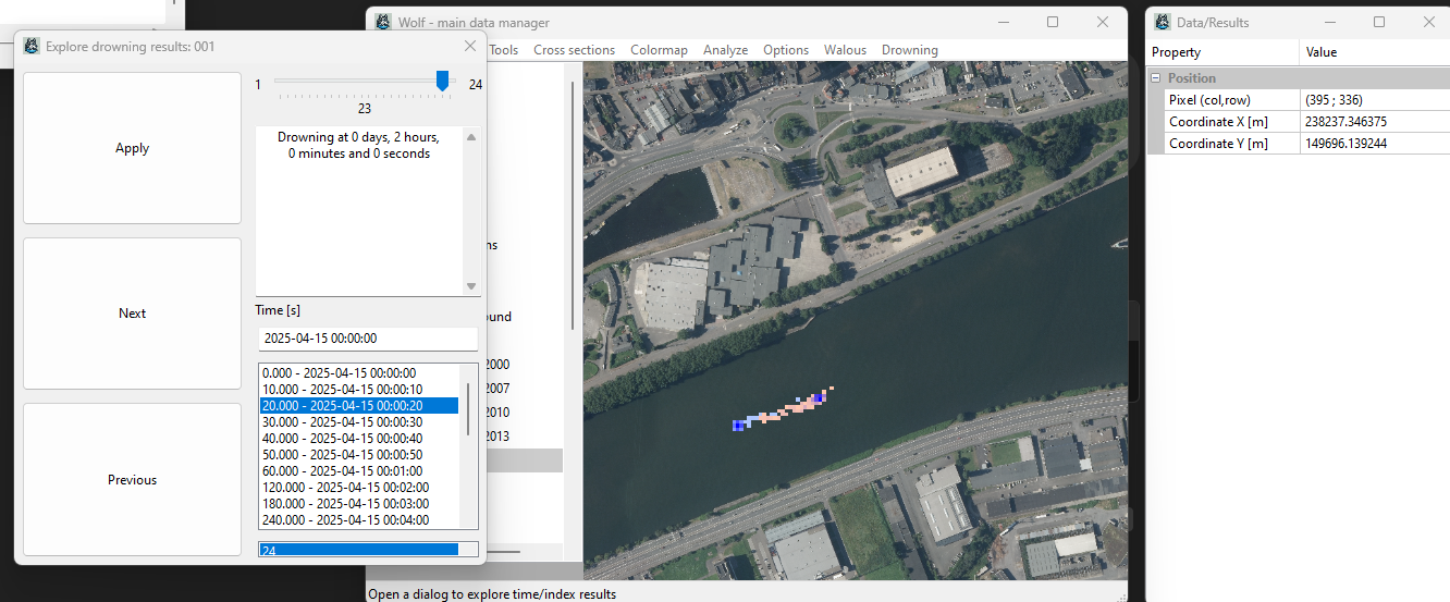
Explore time/index results
This option allows you to select the time where you want to see the results. You can select the time by moving the slider or by selecting a time in the bow. You can edit the initial time of the drowning by changing the time in the box below Time [s]. The time is automatically updated when you select a new time.
Once you have selected the wanted index, press Apply to apply the wanted index on the results. Of course, Previous and Next buttons are available to go to the previous or next index and apply it directly.
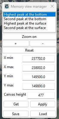
Zoom on hotspots
When selecting this tool, you automatically open a Memory views window. This windows directly contains 4 views: the two highest probability peaks of bodies on the bottom and the same ones but with the bodies at the surface. To get the view, just select it, Apply and Zoom on it.
Get bodies characteristics
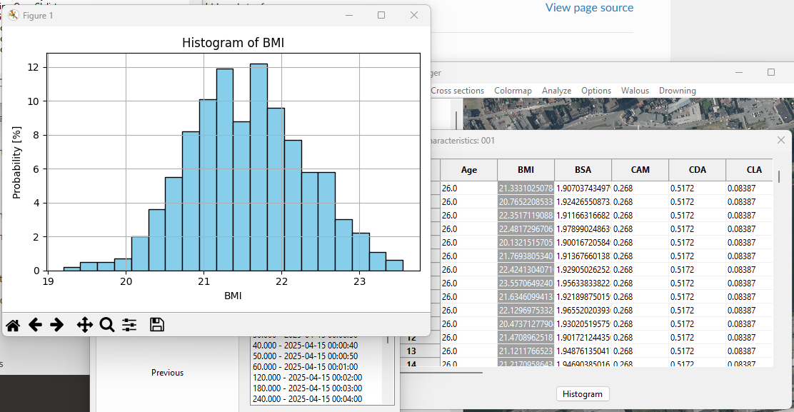
Opens a window with the characteristics of all simulated bodies. The characteristics are displayed in a table whose head is the name of the variable. Everything that is in this window is in the data Human contained in your file Results.npz. This allows you to know the exact characteristics of each of your simulated bodies.
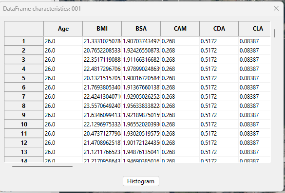
if you select a column by clicking on its name and then you click on the button Histogram, a window opens with a histogram of the selected column.
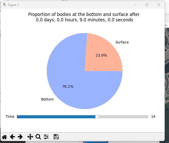
Vertical position proportion
When selected, this option opens a window in which you have a pie chart representing the proportion of bodies on the bottom and at the surface at each time. You can change the time by moving the slider.