WOLF 1D

Note

Mainly based on :

• An Optimized and Scalable Algorithm for the Fast Convergence of Steady 1-D Open-Channel Flows

• Contributions to uncertainty analysis of computational models with application to hydrodynamics and physically-based hydrologic simulations

Mathematical model

Starting from the Navier-Stokes equations for the conservation of mass and momentum, one can derive them in an area-integrated form. These equations are commonly known as Saint-Venant equations:

(1)\[\begin{split}\begin{array}{l} \frac{{\partial A}}{{\partial t}} + \frac{{\partial Q}}{{\partial x}} = {q_l}\\ \frac{{\partial Q}}{{\partial t}} + \frac{\partial }{{\partial x}}\left( {\frac{{{Q^2}}}{A} + g{I_1}} \right) = gA\left( {{S_o} - {S_f}} \right) + g{I_2} + g{I_3} + {u_x}{q_l} \end{array}\end{split}\]

Where \(A\) is the cross-section area, \(Q\) the discharge, \(q_l\) a lateral discharge per unit length, \(g\) the gravity acceleration, \(S_o\) the bed slope, \(S_f\) the friction slope, \(u_x\) the injection velocity according to \(x\) of the lateral discharge, \(I_1\) the pressure integrated on the cross-section and \(I_2\) the force resulting from the pressure on the banks. \(h\) is the water depth, \(h_b\) and \(h_s\) are the distances between the axis \(x\) and, respectively, the riverbed and the free surface.

\[ \begin{align}\begin{aligned}{I_1} = \int_{-h_b}^{h_s} {\left( {{h_s} - \xi } \right)l\left( {x,\xi } \right)d\xi }\\{I_2} = \int_{-h_b}^{h_s} {\left( {{h_s} - \xi } \right)\frac{{\partial l\left( {x,\xi } \right)}}{{\partial x}}d\xi }\end{aligned}\end{align} \]

The \(I_3\) term is added to take into account the fact that a cross-section may present a flat bottom (in the transversal direction). In such a case, the reaction of the pressure on the flat bottom creates a force that acts on the fluid. This reaction occurs when the riverbed presents a longitudinal slope: \(\partial {h_b}/\partial x \ne 0\).

\[{I_3} = h{l_b}\frac{{\partial {h_b}}}{{\partial x}}\]

One can notice that if the cross-section bottom is not flat transversally \(({l_b} = 0)\), the \(I_3\) term vanishes.

In the set of equations, the first one rules the evolution of the cross-section area according to the discharge spatial evolution and the presence of infiltration/exfiltration. The second equation in states that the temporal evolution of the discharge is linked to:

• the spatial change of momentum,

• the spatial change of hydrostatic pressure,

• the bed slope and friction slope,

• the force of reaction coming from the pressure acting on the bed and the banks and,

• a source term to potentially take into account the change of momentum due to the infiltration/exfiltration.

This set of equations, once discretized for numerical solving, is able to reproduce the temporal and spatial evolution of the discharge and cross-section area along a channel according to the major assumption of shallow water equations (SWE): the pressure is considered hydrostatic perpendicular to the flow axis. This assumption can be considered valid in many channel flows when the velocity is mostly directed along the river axis. If 3-D flow patterns exist, the assumption of the SWE are not licit.

For an easier numerical handling of complex cross-sections, the momentum equation in can be written in a non-conservative form (Archambeau 2006). The pressure derivative can be expanded:

\[\begin{split}\begin{array}{c} \frac{\partial }{{\partial x}}\left( {g{I_1}} \right) = g\frac{\partial }{{\partial x}}\left( {\int_{ - {h_b}}^{{h_s}} {\left( {{h_s} - \xi } \right)l\left( {x,\xi } \right)d\xi } } \right)\\ = g\int_{ - {h_b}}^{{h_s}} {\frac{\partial }{{\partial x}}\left[ {\left( {{h_s} - \xi } \right)l\left( {x,\xi } \right)} \right]d\xi } \\ \;\;\, + g\left( {{h_s} - {h_s}} \right)l\left( {x,{h_s}} \right)\frac{{\partial {h_s}}}{{\partial x}} - g\left( {{h_s} + {h_b}} \right)l\left( {x, - {h_b}} \right)\frac{{\partial \left( { - {h_b}} \right)}}{{\partial x}}\\ = g\int_{ - {h_b}}^{{h_s}} {\frac{{\partial \left( {{h_s} - \xi } \right)}}{{\partial x}}l\left( {x,\xi } \right)d\xi } + g\int_{ - {h_b}}^{{h_s}} {\left( {{h_s} - \xi } \right)\frac{{\partial l\left( {x,\xi } \right)}}{{\partial x}}d\xi } - gh{l_b}\frac{{\partial \left( { - {h_b}} \right)}}{{\partial x}}\\ = gA\frac{{\partial {h_s}}}{{\partial x}} + g{I_2} + g{I_3} \end{array}\end{split}\]

Adding up (with their respective signs) the pressure term in its non-conservative form, the forces resulting from the pressure on the banks, the pressure on the bottom of cross-sections and the bed slope results in a single term:

\[\begin{split}\begin{array}{c} \frac{\partial }{{\partial x}}\left( {g{I_1}} \right) - g{I_2} - g{I_3} - gA{S_o} = gA\frac{{\partial {h_s}}}{{\partial x}} + g{I_2} + gh{l_b}\frac{{\partial {h_b}}}{{\partial x}}\\ \;\;\, - g{I_2} - g{I_3} - gA{S_o}\\ = gA\frac{{\partial {h_s}}}{{\partial x}} - gA{S_o}\\ = gA\frac{{\partial {z_s}}}{{\partial x}} \end{array}\end{split}\]

The St-Venant equations in their non-conservative form are:

(2)\[\begin{split}\begin{array}{l} \frac{{\partial A}}{{\partial t}} + \frac{{\partial Q}}{{\partial x}} = {q_l}\\ \frac{{\partial Q}}{{\partial t}} + \frac{\partial }{{\partial x}}\left( {\frac{{{Q^2}}}{A}} \right) + gA\frac{{\partial {z_s}}}{{\partial x}} = - gA{S_f} + {u_x}{q_l} \end{array}\end{split}\]

The non-conservative form of shallow water equations is interesting for a particular reason: the source of movement of the water in a channel naturally appears. Indeed, \(\partial {z_s}/\partial x\), the water surface slope, is explicitly present in (2) while it is not in (1). Moreover, the non-conservative form of shallow water equations showed to perform well in many practical cases, including in the presence of discontinuities (Erpicum, Dewals, Archambeau & Pirotton 2010; Bruwier et al. 2016; Franzini & Soares-Frazão 2016). Further details about the reasons for the good handling of discontinuities by the non-conservative form can be found in (Toro 2000).

The characteristic velocities of equation are obtained from the velocity of the flow \(u\) and the gravity wave speed :

\[\begin{split}\begin{array}{l} {\lambda \_1} = u - c = c\left( {{\rm{Fr}} - 1} \right)\\ {\lambda \_2} = u + c = c\left( {{\rm{Fr}} + 1} \right) \end{array}\end{split}\]

For subcritical flows \((Fr < 1)\), \({\lambda \_1} < 0\) and \({\lambda\_2} > 0\), meaning that an upstream boundary condition and a downstream boundary condition must be set for solving equations . When the flow is supercritical \((Fr > 1)\), both characteristic velocities are positive, meaning that two upstream boundary conditions are required.

Friction modelling

The bottom friction is conventionally modelled with empirical laws, such as the Manning formula, or modern law, such as the Colebrook-White formula. The model enables the definition of a spatially distributed roughness coefficient but this coefficient is unique on each cross-section.

The bottom friction models available in WOLF1D (Fortran) are :

• Manning/Strickler

• Barr-Bathurst

• Colebrrok-White

• Bazin

Grid and numerical scheme

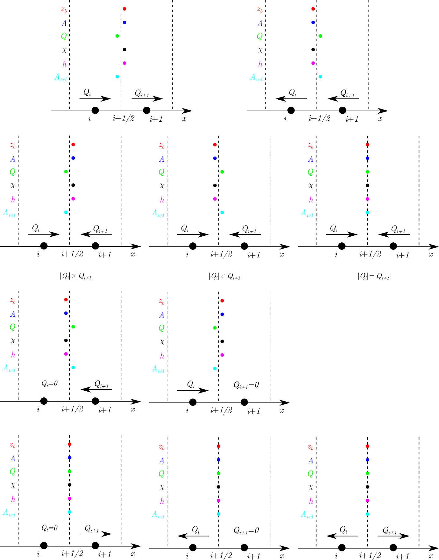
Rivers are spatially discretized according to the finite volume method. The unknowns \(A\) and \(Q\) are associated to the nodes. Properties (such as the water depth) and unknowns are then reconstructed on the borders in order to operate the derivation. This is achieved through the flux vector splitting method (Erpicum, Dewals, Archambeau & Pirotton 2010) which is illustrated below.

The method is based on the sign and value of the discharges \(Q_i\) and \(Q_{i+1}\) on the neighboring nodes \(i\) and \(i+1\). It is independent from the Froude number. In the next Figure, the position of the points represents the direction of the splitting. Basically, the upwinding direction of the discharge \(Q\) and the cross-section area used for computing the velocity in the momentum flux term in , \(A_{vel}\), is upstream. For the bottom elevation \(z_b\), the wet perimeter \(\chi\) and the water depth \(h\), the upwinding direction is downstream. If the discharges \(Q_i\) and \(Q_{i+1}\) are directed toward the border, the upwinding direction is chosen according to the direction of the mean discharge. If both discharges are of the same magnitude, the values are averaged from the two neighboring nodes (this is depicted by a centered point). An averaging is also performed if both discharges go away from the border or if one is directed away from the border and the other is nil. If the discharge is nil in a node and the discharge directed toward the border in the other one, then the upwinding direction is consistent with the classical cases (2 upper schemes in Figure).

At boundary conditions, special values for the discharge and/or water depth are imposed. All other unknowns/properties are reconstructed from the inner node.

Flux vector splitting method

Time discretization

Concerning the time discretization, an explicit Runge-Kutta method is used. The number of steps and the coefficients can be parametrized.

• 1-step (Euler explicit) first order accurate

• 2-step second order accurate – used for transient computations.

• 3-step first order accurate – providing adequate dissipation in time is valuable for steady-state.

For stability reasons, the time step is constrained by the Courant-Friedrichs-Levy condition based on gravity waves. The time step is thus computed as:

\[\Delta t = \min \left( {\frac{{{\rm{NC \kern 2pt }} {\Delta s}}}{{\frac{Q}{A}} + \sqrt \frac{gA}{\frac{\partial A}{\partial z} }}} \right)\]

where NC is the Courant number prescribed by the user. The stable value is depending on the Runge-Kutta algorithm used and the local hydrodynamics, but is lower than 1.

A semi-implicit treatment of the bottom friction term is used, without requiring additional computational costs.

Slight changes in the Runge-Kutta algorithm coefficients allow modifying its dissipation properties and make it suitable for accurate transient computations.

Boundary conditions (external or internal)

For each application, the value of the discharge can be prescribed as an inflow boundary condition. In case of supercritical flow, a water elevation can be provided as additional inflow boundary condition.

Lateral inflow can be prescribed as a discharge in \(m^3s^{-1}\). The discharge per unit length will be automatically computed.

All discharges can be a function of time, linearly interpolated or stewpwise.

The outflow boundary condition may be a water surface elevation, a Froude number or no specific condition if the outflow is supercritical.

Topography data

Cross-sections can be defined by the user. The topography data can be provided as a 3D polyline, a look-up table \((h-A-\chi)\) or as a function (rectangular, circlular, trapzoidal).

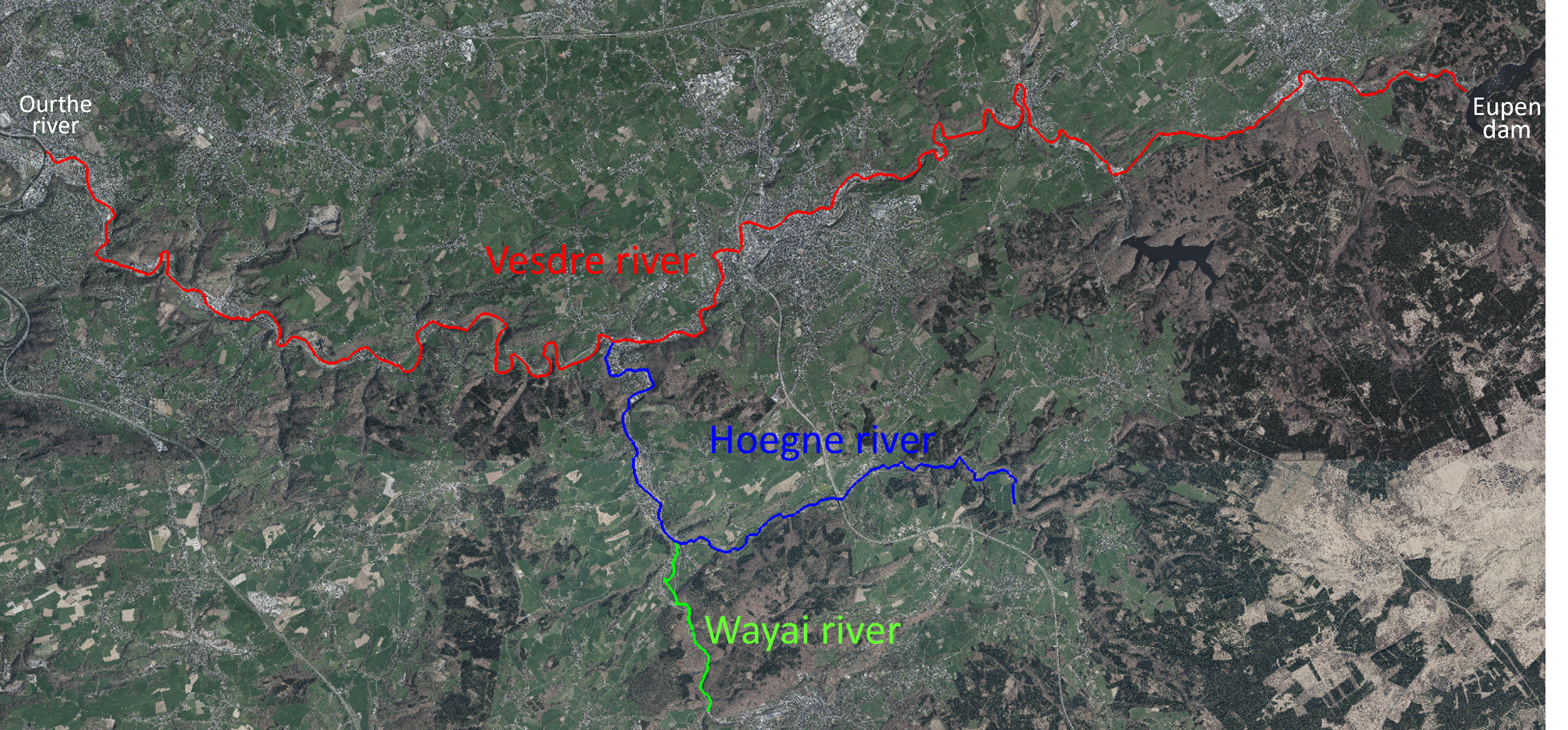
The cross-sections can be geolocalized as wel as the rivers axis.

Since 2000, high resolution, high accuracy topographic datasets have become increasingly available for inundation modelling in a number of countries. In Belgium, a data collection programme using airborne laser altimetry (LIDAR) has generated high quality topographic data covering the floodplains of most rivers in the southern part of the country (2002), the whole Region (2013-2014, 2021-2022) and more recently a combined data including bathymetry using green Lidar.

Wolf1D can use these data to extract the cross-sections.

Modified 1-D model for fast water profile computation

The use of an initial condition is a prerequisite for an unsteady simulation. In many situations, this initial situation is a converged steady flow. For other applications, only a steady solution is the desired output.

The computation of a steady flow is of main importance in the hydraulic field. A fast computation is the key in order to be able to perform a large number of simulations in a reasonable amount of time.

Equation

Assuming a steady flow leads to temporal derivatives equal to 0 in :

\[\begin{split}\begin{array}{l} \frac{{\partial Q}}{{\partial x}} = {q_l}\\ \frac{\partial }{{\partial x}}\left( {\frac{{{Q^2}}}{A} + g{I_1}} \right) = gA\left( {{S_o} - {S_f}} \right) + g{I_2} + {u_x}{q_l} \end{array}\end{split}\]

The first expression means that the discharge is known along the channel thanks to the boundary conditions and lateral discharge injections. It means that a single equation remains with a single unknown \(A\). In order to keep the same numerical scheme as the one used for the unsteady system, Kerger et al. (2011) add a pseudo-temporal term to equation :

\[\beta \frac{{\partial A}}{{\partial \tau }} + \frac{\partial }{{\partial x}}\left( {\frac{{{Q^2}}}{A} + g{I_1}} \right) = gA\left( {{S_o} - {S_f}} \right) + g{I_2} + {u_x}{q_l}\]

where \(\tau\) is a pseudo-time and \(\beta = - {\rm{sign}}\left( Q\right)\) as explained in (Kerger et al. 2011). This is chosen by analyzing the characteristic velocity of equation :

\[\lambda = \frac{{{c^2} - {u^2}}}{\beta } = \frac{{{c^2}\left( {1 - {\rm{F}}{{\rm{r}}^2}} \right)}}{\beta }\]

where \(c\) is the wave celerity. In subcritical flows \((Fr < 1)\), and the sign of \(\lambda\) is the sign of \(\beta\). If \(Fr > 1\), then \({\rm{sign}}\left( \lambda \right) = - {\rm{sign}}\left( \beta \right)\). For critical flows \((Fr = 1)\), the characteristic velocity is 0, independently from \(\beta\). In order to keep some form of consistency with the general model, if we choose \(\beta = -{\rm{sign}}\left( Q \right)\), an upstream boundary condition is required when \(Fr > 1\) and a downstream boundary condition is required when \(Fr < 1\). This is equivalent to the position of the water depth boundary condition for the numerical resolution of the general 1-D set of equations.

Such as the transformation operated on equations to get equations, equation can be written in its non-conservative form:

\[\beta \frac{{\partial A}}{{\partial \tau }} + \frac{\partial }{{\partial x}}\left( {\frac{{{Q^2}}}{A}} \right) + gA\frac{{\partial {z_s}}}{{\partial x}} = - gA{S_f} + {u_x}{q_l}\]

With a single boundary condition and a discharge distributed in the river stretch, by solving equation we are able to determine the cross-section area (and subsequently water depth) all along the river. The solving is performed according to the same numerical scheme as the one used for the general unsteady model which was shown to be unconditionally stable (Kerger et al. 2011).

For a node \(i\), equation is discretized in finite volumes as:

\[\frac{{Q_{i + 1/2}^2/{A_{i + 1/2}} - Q_{i - 1/2}^2/{A_{i - 1/2}}}}{{\Delta x}} + g{A_i}\left( {\frac{{{z_{s,i + 1/2}} - {z_{s,i - 1/2}}}}{{\Delta x}} + {S_{f,i}}} \right) - {u_{x,i}}{q_{l,i}} \approx - \beta \frac{{\partial A}}{{\partial \tau }}\]

where \(\Delta x\) is the spatial discretization step and subscripts refer to the position of variables values.

For the sake of clarity, we consider \(Q > 0\) and a constant reconstruction of the flux at finite volume boundaries to explicate the numerical scheme. When applying the considered upwinding directions for a node \(i\) not located next to a boundary, equation is equivalent to:

\[\frac{{Q_i^2/{A_i} - Q_{i - 1}^2/{A_{i - 1}}}}{{\Delta x}} + g{A_i}\left( {\frac{{{z_{s,i + 1}} - {z_{s,i}}}}{{\Delta x}} + {S_{f,i}}} \right) - {u_{x,i}}{q_{l,i}} = \frac{{\partial A}}{{\partial \tau }}\]

For the node located at the downstream boundary \((i = N - 1)\), if a weak water level boundary condition \(z_{s,BC}\) is imposed at the border, equation becomes:

\[\frac{{Q_{N - 1}^2/{A_{N - 1}} - Q_{N - 2}^2/{A_{N - 2}}}}{{\Delta x}} + g{A_{N - 1}}\left( {\frac{{{z_{s,BC}} - {z_{s,N - 1}}}}{{\Delta x}} + {S_{f,N - 1}}} \right) - {u_{x,N - 1}}{q_{l,N - 1}} = \frac{{\partial A}}{{\partial \tau }}\]

Without a boundary condition imposed on the value of \(z_s\) at the external border, a nil \(z_s\) gradient is imposed and equation becomes:

\[\frac{{Q_{N - 1}^2/{A_{N - 1}} - Q_{N - 2}^2/{A_{N - 2}}}}{{\Delta x}} + g{A_{N - 1}}{S_{f,N - 1}} - {u_{x,N - 1}}{q_{l,N - 1}} = \frac{{\partial A}}{{\partial \tau }}\]

At the upstream node (\(i = 0\)), if a weak boundary condition of the water level is imposed at the border, equation becomes:

\[g{A_0}\left( {\frac{{{z_{s,1}} - {z_{s,BC}}}}{{\Delta x}} + {S_{f,0}}} \right) - {u_{x,0}}{q_{l,0}} = \frac{{\partial A}}{{\partial \tau }}\]

Without a boundary condition at the upstream border, equation becomes:

\[g{A_0}\left( {\frac{{{z_{s,1}} - {z_{s,0}}}}{{\Delta x}} + {S_{f,0}}} \right) - {u_{x,0}}{q_{l,0}} = \frac{{\partial A}}{{\partial \tau }}\]

Original solving strategy

Solving this equation allows time saving in computation since the number of equations and unknowns is reduced.

In order to gain more time, two additional strategies are implemented:

• an Anderson accelerator is used in order to promote fast convergence.

• the computation is performed only on a sliding part of the full domain.

Anderson acceleration

Numerically solving a non-linear system can be performed by different means, including Newton’s method and Broyden’s method (Broyden 1965). Newton’s method consists in computing a Jacobian matrix (numerically when an analytical evaluation is not possible) at each iteration in order to converge to a local optimum. Broyden’s method is similar to Newton’s method except that it computes the entire Jacobian matrix only at the first iteration and then updates it for the following steps.

More sophisticated methods exist in order to solve non-linear systems faster, such as the Jacobian-free Newton-Krylov method (Knoll & Keyes) and Anderson acceleration (Anderson 1965). The Anderson acceleration method uses the results from successive iterations in order to adapt the new approximation. Walker & Ni (2011) showed that this method can be considered equivalent to the well-known GMRES method (Saad & Schultz 1986) when applied to linear systems. The nonlinear Krylov acceleration (NKA) (Carlson & Miller 1998a; Carlson & Miller 1998b), which is similar to Anderson acceleration, showed to be more efficient in some applications than more recent methods such as the Jacobian-Free Newton-Krylov method (Calef et al. 2013). NKA is used for a faster convergence of our pseudo-time model.

Sliding domain

In order to decrease the computational cost, a second strategy was designed. It consists in reducing the size of the computation domain and slide it along the river stretch in order to converge the cross-section areas from downstream to upstream. The main principle is explained graphically in the next Figure. Starting from the downstream limit, a partial computation domain slides gradually toward the upstream limit. When the most upstream node is converged, a final computation of the entire domain is performed.

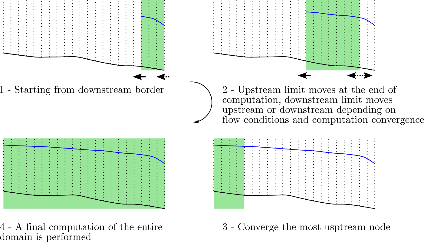
Principle of the sliding domain (green area). It starts from the downstream border et slides gradually toward the upstream limit.

The development of this strategy has arisen from the long history of numerical hydrodynamics in various flow regimes. Indeed, many flows that are solved for rivers are subcritical \((Fr < 1)\) at downstream and upstream boundary conditions. In such a situation, the cross-section area information is propagated from downstream to upstream. For a fixed flow direction, the upwinding direction of the numerical scheme takes all unknowns and properties (except those linked to the discharge and velocity) downstream. This means that when a new node is computed, it depends only on the downstream nodes (see Figure 33). It should be noticed that when a node \(i\) is added, the upstream border of node \(i +1\) produces a change in the upwinding direction of property \(Q\) and the unknown \(A_vel\) (cross-section area used to compute the velocity). The node \(i + 1\), which was supposed to be converged, undergoes a new convergence process that indirectly affects nodes \(i + 2\), \(i + 3\). Theoretically, all the nodes located downstream of node \(i\) should be kept in the computational domain. However, for better computation efficiency, it was chosen to remove a node from the computation domain if the rate of change of the cross-section area was lower than some threshold. When the most upstream node is converged, a last convergence process is performed for the whole domain, ensuring that all nodes have reached a stable value. Indeed, as stated earlier, all nodes should be theoretically kept in the computation domain since newly added upstream nodes affect downstream nodes. This final step ensures that all nodes are converged with a residual \(\left\| {\partial A/\partial \tau }\right|\), denoted \(\xi\), low enough.

Numerical scheme used at the boundary of the sliding domain

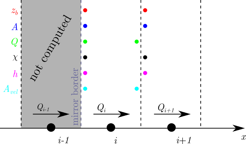
The boundary condition on the border between the node \(i\) and node \(i – 1\) is called a “mirror border”. On this border, all the unknowns and properties are reconstructed from the computed inner node. It is not considered as a boundary border since no discharge nor water depth are imposed. This method is equivalent to reproducing the node \(i\) in \(i – 1\), like a mirror.

When a new node is added to the computation domain, a first estimation of the cross section area is performed in order to get an overall faster convergence. The technique used consists in estimating the cross section area of node \(i\) in order to verify the pseudo-time momentum equation for node \(i\). If the source term is nil, then we should have

\[\begin{split}\begin{array}{r} \frac{\partial }{{\partial x}}\left( {\frac{{{Q^2}}}{A} + {z_s}} \right) = 0\\ \Leftrightarrow \frac{\partial }{{\partial x}}\left( {\frac{{{Q^2}}}{A}} \right) + \frac{{\partial {z_s}}}{{\partial x}} = 0 \end{array}\end{split}\]

Since the discharge \(Q\) and the cross section area used for the velocity computation, \(A_vel\) are reconstructed from node \(i\) for both borders, the only solution is to equal the water levels \(z_s\):

\[\begin{split}\begin{array}{r} \frac{\partial }{{\partial x}}\left( {\frac{{{Q^2}}}{A}} \right) + \frac{{\partial {z_s}}}{{\partial x}} = 0\\ \Leftrightarrow \frac{{\partial {z_s}}}{{\partial x}} = 0 \end{array}\end{split}\]

This solution may lead to inconsistency for steep slopes and low water levels. This is why, when the friction source term is nil, the water depth is simply copied to the newly added node.

When this source term is not nil, a Newton-Raphson iteration process is implemented in order to reach an equilibrium between the spatial derivative and the source term. The first estimation of the cross section area of node \(i\) is the cross section area of node \(i+1\). Then, the cross section area is slightly perturbed by \(\Delta A\). Two values

\[\begin{split}\begin{array}{l} {f_1} = \frac{\partial }{{\partial x}}\left( {\frac{{{Q^2}}}{A} + {z_s}} \right) + gA{S_f}\\ {f_2} = \frac{\partial }{{\partial x}}\left( {\frac{{{Q^2}}}{{\left( {A + \Delta A} \right)}} + {z_s}} \right) + g\left( {A + \Delta A} \right){S_f} \end{array}\end{split}\]

are computed. The new trial value of \(A_new\) is based on the previous results:

\[{A_{new}} = A - \frac{{{f_1}}}{{\frac{{{f_2} - {f_1}}}{{\Delta A}}}}\]

This procedure is performed until \(f_1\) is lower than some threshold.

As stated earlier, the method described here was designed in the frame of subcritical flows. In order to be able to deal with a larger range of flow regimes, some adaptations were made. When a supercritical node is detected downstream (let say at position \(m\)), it is not computed and the computation domain is extended until a subcritical node is found upstream (let say at position \(n\)). Then, the domain starting from \(m\) to \(n\) is computed and converged. If this technique was not used a boundary condition problem would occur. Indeed, a supercritical flow requires an upstream BC since the characteristic velocity is directed downstream.

A general view of the algorithm is given. It shows that after initialization, a main loop is started. It consists in computing only a part of the entire domain, using the evolutionary domain concept explained before. The computation domain span evolves in the “Vary domain span” box.

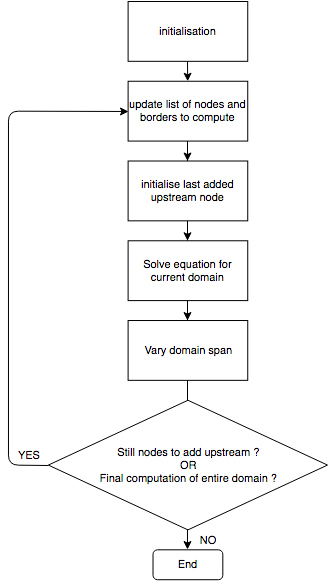
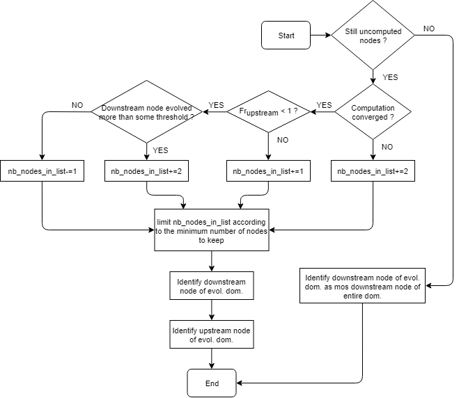
First, a check is made to know if some nodes still not computed. Indeed, when all the nodes are computed at least once, a final computation is done on the entire domain in order to ensure a final convergence. If some nodes still have to be added to the computation domain, several checks are made in order to identify the status of the computation:

• If the computation is identified as not converged, the computation domain is increased by adding the downstream and upstream nodes (+ 2 nodes)

• If the flow upstream is supercritical, then the downstream limit is not modified but a node is added upstream (+ 1 node)

• If the most downstream node of the computation domain changed more than some threshold, then the domain is extended downstream as well as upstream (+ 2 nodes), otherwise a node is removed from the domain (- 1 node)

• When the number of nodes to keep is known (and adjusted to agree with the minimum number of nodes to keep in the list), the upstream and downstream nodes of the computation domain are pointed and a new iteration of the main loop can begin.

Combination of solving strategies

The combined use of the sliding domain and NKA involves several specific considerations. The use of NKA is implemented in the code with a safety coefficient that deactivates this optimizing technique in some cases. Indeed, it was experienced that NKA could lead to some instabilities when there was a sudden change in the cross-section area. This behavior is due to the assumption in NKA that the Jacobian matrix is constant and invertible locally (Calef et al. 2013; Wang et al. 2018). Problems with this assumption were encountered in several situations. We found that the main one is when cross section areas of the two most upstream nodes are too different. Our experience showed that the accelerator should be deactivated when:

\[\left\| {{A_{i + 1}} - {A_i}} \right\| > \eta {A_{i + 1}}\]

where \(A_i\) and \(A_{i+1}\) refer to the cross-section area of the node \(i\) and \(i+1\) as depicted in the Figure, \(0 < \eta \le 1\) is the safety coefficient. It has to be defined in order to reach optimal computation times.

Note

More information about this can be found in

• Louis Goffin Thesis

• An Optimized and Scalable Algorithm for the Fast Convergence of Steady 1-D Open-Channel Flows

Fortran code

WOLF1D is coded in Object-Oriented Fortran and compiled as an executable using Intel compiler. The code is parallelized using OpenMP.

The code is available on request.

First tutorial

Une vidéo illustrative des opérations de base est disponible :

Exemple

Représentation du domaine de calcul

Visualisation des sections transversales - superposition aux orthophotoplans (Walonmap)

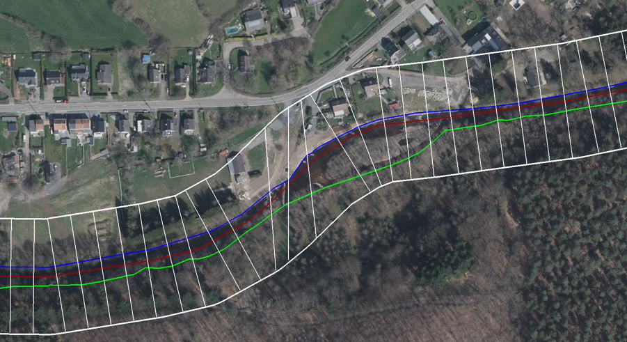
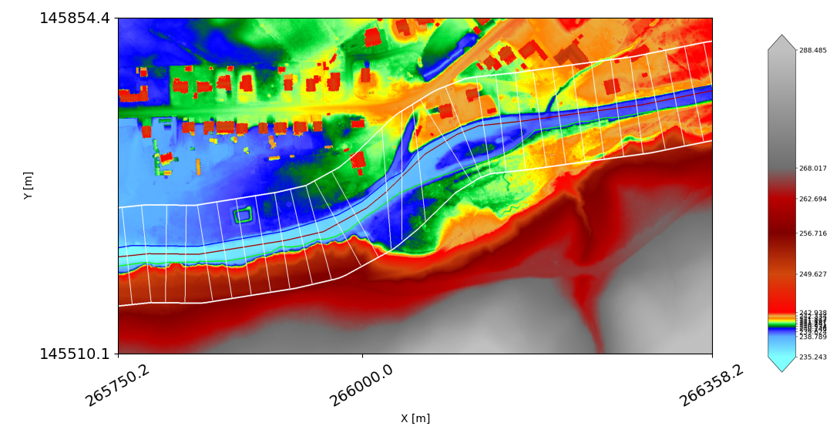
Visualisation des sections transversales - superposition à la données Lidar

Exemple d’une fenêtre de visualiasation des résultats