Shields parameter

The Shields parameter is a hydro-sedimentary parameter.

It is defined by the following formula:

\[\theta = \frac{\tau}{\tau_c}\]

where:

\(\theta\) is the Shields parameter,
\(\tau\) is the shear stress exerted by water on the river bed,
\(\tau_c\) is the critical shear stress, i.e. the minimum shear stress required to initiate sediment motion.

The Shields parameter is used to assess the stability of sediments in a watercourse. It determines whether the hydraulic conditions are sufficient to set sediment particles in motion. A \(\theta\) greater than 1 indicates that conditions are sufficient to initiate sediment motion, while a \(\theta\) less than 1 indicates that they are not.

The Shields diagram

The Shields diagram is a graph that represents the Shields parameter as a function of the Reynolds number and the Froude number. It is used to visualize the hydraulic conditions in a watercourse and to assess sediment stability.

alt text

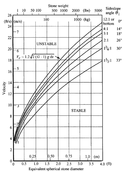
Source: Van Rijn (1984), Sediment Transport, Part I: Bed Load Transport, Journal of Hydraulic Engineering, ASCE, 110(10):1431-1456.

Python implementation

In the wolfhece package, tools are available through the pyshields module to compute the Shields parameter and plot the Shields diagram in various forms.

References

Some useful references for further reading:

Telemac-Mascaret
Yalin, Ferraira da Silva (2001), Fluvial Processes, IAHR Monograph
Fredsoe, Jorgen and Deigaard Rolf. (1992). Mechanics of Coastal Sediment. Sediment Transport. Advanced Series on Ocean Engineering - Vol. 3. World Scientific. Singapore.
Madsen, Ole S., Wood, William. (2002). Sediment Transport Outside the Surf Zone. In: Vincent, L., and Demirbilek, Z. (editors), Coastal Engineering Manual, Part III, Combined wave and current bottom boundary layer flow, Chapter III-6, Engineer Manual 1110-2-1100, U.S. Army Corps of Engineers, Washington, DC.
Nielsen, Peter. (1992). Coastal Bottom Boundary Layers and Sediment Transport. Advanced Series on Ocean Engineering - Vol. 4. World Scientific. Singapore.

Importing modules

[1]:

try:
    required_version = '2.2.30'
    from wolfhece import is_enough
    is_enough(required_version)

    import timeit
    import matplotlib.pyplot as plt

    from wolfhece.pyshields import RHO_SEAWATER, RHO_PUREWATER, RHO_SEDIMENT, get_shields_cr, get_d_cr
    from wolfhece.pyshields import shieldsdia_dim, shieldsdia_dstar, shieldsdia_sadim # routines graphiques
    from wolfhece.pyshields import get_d_cr_susp, get_transport_mode # suspension
except ImportError as e:
    print(f"Import error: {e}")
    print("Please ensure that the wolfhece package is installed and up to date.")
    print(f"Minimal version required: {required_version}")

Critical Shields parameter

Several formulations exist.

The which parameter selects the function via its index in the list [(get_sadim, get_psi_cr), (get_dstar, get_psi_cr2), (get_dstar, get_psi_cr3)]:

which = 0 → (get_sadim, get_psi_cr) — reference
which = 1 → (get_dstar, get_psi_cr2) — reference
which = 2 (default) → (get_dstar, get_psi_cr3) — reference: Fluvial Processes, IAHR 2001, pp 6-9

[3]:

print("Default formula  is which == 2 (get_dstar, get_psi_cr3)\n")
for which in [0, 1, 2]:
    res = get_shields_cr(d = 0.2e-3, rho = RHO_PUREWATER, which=which)
    print(f"Result for which = {which}")
    # critical_shear_velocity, tau_cr, xadim_val, psicr
    print(f"Critical shear velocity: {res[0]:.4f} m/s, Tau_cr: {res[1]:.4f} N/m², Xadim_val: {res[2]:.4f}, Psi_cr: {res[3]:.4f}\n")

Default formula  is which == 2 (get_dstar, get_psi_cr3)

Result for which = 0
Critical shear velocity: 0.0128 m/s, Tau_cr: 0.1649 N/m², Xadim_val: 2.8449, Psi_cr: 0.0509

Result for which = 1
Critical shear velocity: 0.0127 m/s, Tau_cr: 0.1606 N/m², Xadim_val: 5.0592, Psi_cr: 0.0496

Result for which = 2
Critical shear velocity: 0.0139 m/s, Tau_cr: 0.1942 N/m², Xadim_val: 5.0592, Psi_cr: 0.0600

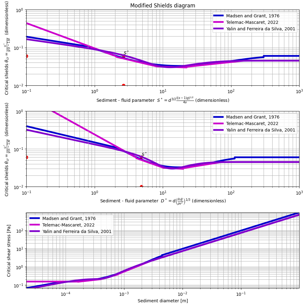
Diagrams

The Shields diagram can be plotted in several forms:

shieldsdia_dstar: Shields parameter vs. dimensionless grain diameter (d*) — dimensionless axes
shieldsdia_sadim: Shields parameter vs. dimensionless parameter s_adim — dimensionless axes
shieldsdia_dim: Shields parameter vs. hydraulic diameter — dimensional axes

The s_psicr and dstar_psicr arguments allow plotting a specific point on the diagram. They are tuples of the form (value, psicr) where value is the parameter value to plot and psicr is the critical Shields parameter value.

[4]:

fig, ax = plt.subplots(3,1)

s = RHO_SEDIMENT / RHO_PUREWATER # ratio of sediment density to water density
shear_cr, tau_cr, xadim, psi_cr =  get_shields_cr(d = 0.2e-3, rho = RHO_PUREWATER, which = 2)

shieldsdia_sadim(s_psicr=(s,psi_cr), figax=(fig,ax[0]))
shieldsdia_dstar(s_psicr=(s,psi_cr), figax=(fig,ax[1]))
shieldsdia_dim(figax=(fig,ax[2]))

ax[0].set_title('Modified Shields diagram')
fig.set_size_inches(10,10)
fig.tight_layout()
fig.show()

C:\Users\pierre\AppData\Local\Temp\ipykernel_12488\4240051310.py:13: UserWarning: FigureCanvasAgg is non-interactive, and thus cannot be shown
  fig.show()

Determining the critical parameter from the sediment diameter

In this approach, the formula is explicit. This poses no particular difficulty.

Determining the critical sediment diameter from the shear stress

In this approach, the formula is implicit. A numerical method is therefore required to find the critical sediment diameter.

This is implemented in the get_d_cr function, which uses the brenth method by default to find the root. It additionally returns the diameter according to the Izbash formula.

alt text

source

Example with Manning-Strickler

[5]:

dcr_shields, dcr_izbach = get_d_cr(q = 10.,
                                   h = 2.,
                                   K = 25.)

print(f"Critical diameter (Shields): {dcr_shields:.4f} m, Critical diameter (Izbach): {dcr_izbach:.4f} m")

Critical diameter (Shields): 0.4276 m, Critical diameter (Izbach): 0.5363 m

Example with Colebrook-White

It is also possible to compute the critical sediment diameter as a function of the shear stress and a roughness height to be used in the Colebrook-White formula.

[6]:

dcr_shields, dcr_izbach = get_d_cr(q = 10.,
                                   h = 2.,
                                   K = 0.05,
                                   friction_law='Colebrook')

print(f"Critical diameter (Shields): {dcr_shields:.4f} m, Critical diameter (Izbach): {dcr_izbach:.4f} m")

Critical diameter (Shields): 0.1396 m, Critical diameter (Izbach): 0.5363 m

Suspension and transport mode

It is also possible to compute:

the critical diameter for 50 % suspension entrainment
the sediment transport mode

Note: currently only the Manning-Strickler friction law is implemented, but extending to others is straightforward.

[7]:

dsusp = get_d_cr_susp(q = 10.,
                      h = 2.,
                      K = 25.,
                      rhom = RHO_SEDIMENT,
                      rho = RHO_PUREWATER)

print(f"Critical diameter for suspension: {dsusp:.4f} m")

Critical diameter for suspension: 0.0152 m

[8]:

from wolfhece.pyshields import BED_LOAD, SUSPENDED_LOAD_100, SUSPENDED_LOAD_50, WASH_LOAD

mode = get_transport_mode(d = 0.2e-3,
                          q = 10.,
                          h = 2.,
                          K = 25.,
                          rhom = RHO_SEDIMENT,
                          rho = RHO_PUREWATER)

if mode == BED_LOAD:
    print("Bed load transport")
elif mode == SUSPENDED_LOAD_100:
    print("Suspended load transport at 100%")
elif mode == SUSPENDED_LOAD_50:
    print("Suspended load transport at 50%")
elif mode == WASH_LOAD:
    print("Wash load transport")

Wash load transport