Simple triangulation

A triangulation is defined by a list of vertices (as numpy array - shape (n,3)) and an enumeration of triangles (by indices).

It can be created/imported from DXF or GLTF/GLB files.

Default file format is .tri, a binary Wolf format.

# import _add_path # this line can be removed if wolfhece is installed in the python path

from wolfhece import __version__
assert __version__ > "2.2.8", "Please update wolfhece to at least 2.2.8, you have " + __version__

import numpy as np
import matplotlib.pyplot as plt

from wolfhece.PyVertexvectors import Triangulation

Basics example

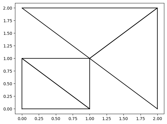
# Simple example of a triangulation with 3D points
pts= np.array([[0., 0., 2.],
               [1., 0., 3.],
               [0., 1., 4.],
               [1., 1., 5.],
               [2., 2., 0.],
               [2., 0., 0.],
               [0., 2., 0.]])

triangles = np.array([[0, 1, 2],
                        [1, 3, 2],
                        [5, 4, 3],
                        [3, 4, 6]])
tri = Triangulation(pts=pts, tri=triangles)

fig, ax = plt.subplots()
tri.plot_matplotlib(ax)

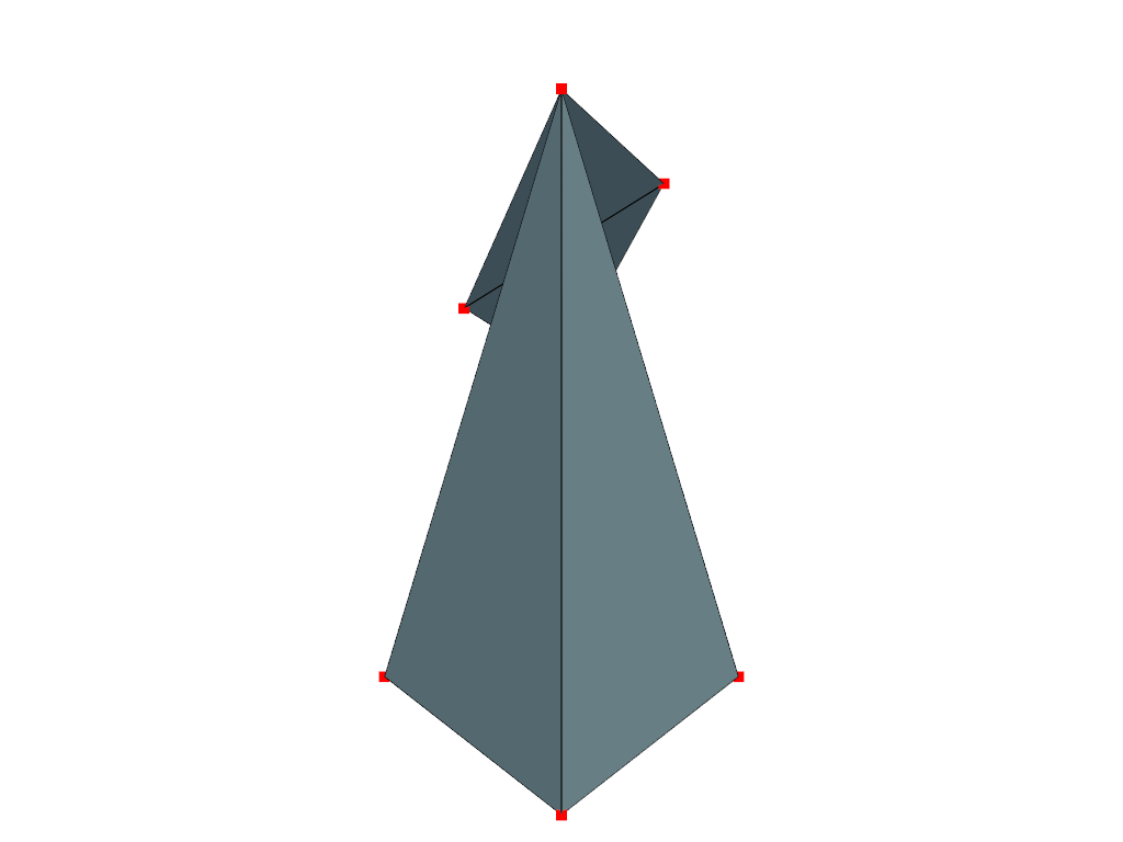
Plot with Pyvista

See https://pyvista.org/

import pyvista as pv

# Create a PyVista plotter object
plotter = pv.Plotter()
# Add the triangulation to the plotter
plotter.add_mesh(tri.as_polydata(), show_edges=True, color='lightblue')
# Add the points to the plotter
plotter.add_points(pts, color='red', point_size=10)
# Show the plot
plotter.show()

d:\ProgrammationGitLab\python3.10\lib\site-packages\pyvista\jupyter\notebook.py:34: UserWarning: Failed to use notebook backend:

No module named 'trame'

Falling back to a static output.
  warnings.warn(

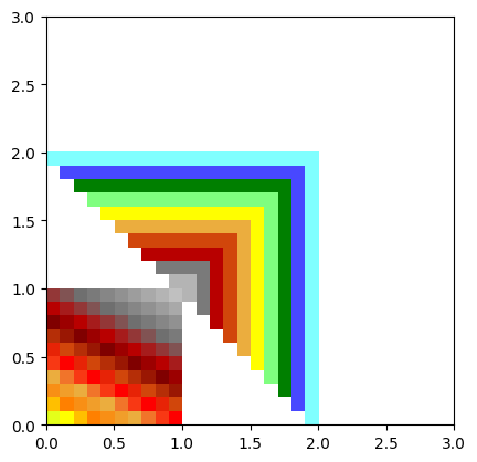
Interpolate on array

from wolfhece.wolf_array import WolfArray, header_wolf

h = header_wolf()
h.set_resolution(.1, .1)
h.set_origin(0., 0.)
h.shape = 30, 30

wa = WolfArray(srcheader=h)
wa.nullvalue = 1.
wa.interpolate_on_triangulation(tri.pts, tri.tri)
wa.plot_matplotlib()

(<Figure size 640x480 with 1 Axes>, <Axes: >)

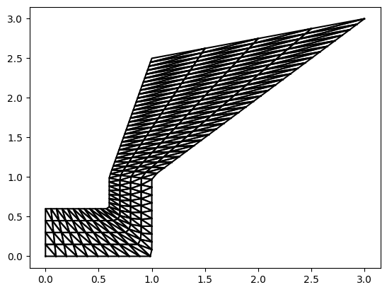
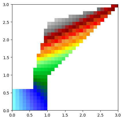
Creation from vectors/zone

from wolfhece.PyVertexvectors import zone, vector, wolfvertex

# Create a zone object
z = zone()

# Create vector objects
v1 = vector()
v2 = vector()

v1.add_vertices_from_array(np.array([[0., 0., 3.],
                                     [1., 0., 4.],
                                     [1., 1., 5.],
                                     [3., 3., 7.]]))

v2.add_vertices_from_array(np.array([[0., 0.6, 3.],
                                     [0.6, 0.6, 4.],
                                     [0.6, 1., 5.],
                                     [1., 2.5, 8.]]))

z.add_vector(v1, forceparent=True)
z.add_vector(v2, forceparent=True)

# update the lengths of the vectors
# (this is necessary to calculate the length of the vectors in 2D and 3D)
v1.update_lengths()
v2.update_lengths()

print('length of vector 1:', v1.length2D)
print('length of vector 2:', v2.length2D)

tri2 = z.create_multibin(50, 3) # 50 regular steps along the vectors, 5 intermediate steps in-between

fig, ax = plt.subplots()
tri2.plot_matplotlib(ax)

length of vector 1: 4.82842712474619
length of vector 2: 2.5524174696260022

wa2 = WolfArray(srcheader=h)
wa2.nullvalue = 0.  # set null value to 0.
wa2.array[:,:] = 0. # set all values to 0.
wa2.interpolate_on_triangulation(tri2.pts, tri2.tri) # interpolate on the new triangulation
wa2.plot_matplotlib() # plot the interpolated values, nullvalue will be masked in the plot

print(wa2.array[0,-1])

--

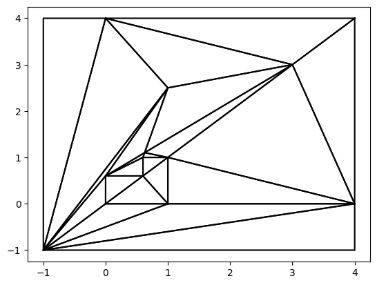
Constrained Delaunay Triangulation

We can create a triangulation from a set of points using the Delaunay triangulation algorithm. This is useful for generating a mesh from scattered data points.

Internally, we use the great “triangle” library (https://rufat.be/triangle/index.html - https://www.cs.cmu.edu/~quake/triangle.html)

To create a constrained triangulation from a zone, it is necessary to define at least one polygon that specifies the triangulation area.

Other vectors will be used as triangulation constraints.

Be careful, vectors must not be self-intersecting and must not cross each other. Otherwise, triangulation may fail and/or corrupt memory/jupyter kernel.

# add a new vector to the zone - as external vector
external = vector()
external.add_vertices_from_array(np.array([[-1., -1., 0.],
                                         [4., -1., 0.],
                                         [4., 4., 0.],
                                         [-1., 4., 0.],
                                         [-1., -1., 0.]
                                        ]))
z.add_vector(external, forceparent=True)

tri_del = z.create_constrainedDelaunay(nb = 0) # use vector as it is

fig, ax = plt.subplots()
tri_del.plot_matplotlib(ax)

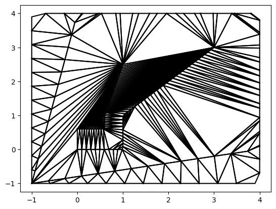
tri_del2 = z.create_constrainedDelaunay(nb = 50) # subdivide each vector into 50 steps - intermediate vertices (corners) not necessary respected

fig, ax = plt.subplots()
tri_del2.plot_matplotlib(ax)