Creating a 2D Simulation with CPU model with turbulence via script
To create a 2D simulation, you need to:
Set simulation name and working directory and check
.climodel availabilityCreate a new 2D simulation as an instance of
prev_sim2DDefine the problem geometry (mesh resolution, channel dimensions) and boundary conditions
Define a vectorial contour/polygon to outline the working area and add blocks (obstacles)
Define a magnetic grid, set the contour, and create the mesh
Set the simulation parameters
Get boundary cells and set boundary conditions
Define initial conditions and other simulation parameters (topography, water depth, friction)
Final checks and save the simulation
Run the simulation
run_wolfcli
And…
Access the results
Visualize the results
Generate an animation
Preliminary steps
Import modules
[ ]:
# general modules
import os
import numpy as np
import matplotlib.pyplot as plt
import matplotlib.animation as animation
from pathlib import Path
from IPython.display import HTML, Image
from datetime import datetime as dt
from datetime import timezone as tz
from datetime import timedelta as td
# WOLF modules
from wolfhece.mesh2d.wolf2dprev import prev_sim2D
from wolfhece.PyVertexvectors import vector, wolfvertex
from wolfhece.wolf_array import WolfArray, WolfArrayMB, header_wolf
from wolfhece.mesh2d.cst_2D_boundary_conditions import BCType_2D
from wolfhece.wolfresults_2D import Wolfresults_2D
from wolfhece.wolfresults_2D import views_2D, getkeyblock
Set simulation name and directory
[2]:
simulation_name = 'tutorial_2D'
curdir = Path(os.getcwd())
print(f'Current directory: {curdir}')
Current directory: d:\ProgrammationGitLab\HECEPython\Floating_Debris\WOLF_simulations
[3]:
outdir = curdir / simulation_name
outdir.mkdir(exist_ok=True) # create output folder
print(f'Simulation path: {outdir}; name: {outdir.name}')
Simulation path: d:\ProgrammationGitLab\HECEPython\Floating_Debris\WOLF_simulations\tutorial_2D; name: tutorial_2D
Check code availability
Return full path to the executable. It is recommended to have the executable in the directory where this notebook is stored.
[4]:
wolfcli = prev_sim2D.check_wolfcli() # check if wolfcli is present in the current directory
if wolfcli:
print('Code found: ', wolfcli)
else:
print('Code not found!')
Code found: wolfcli.exe
Create new 2D simulation
clear=True allows you to delete the files from the previous simulation, if existing.logging.warning is emitted because no file was found. This is normal, as you just created the simulation![5]:
new_dir = outdir / f'{simulation_name}'
newsim = prev_sim2D(fname=new_dir, clear=True)
WARNING:root:No infiltration file found
Define problem geometry and boundary conditions
Definition Method
Channel configuration:

Geometry
Specify the mesh size (dx, dy), coordinates of the origin (origx, origy), channel dimensions (Lx, Ly), and slope.
[6]:
dx, dy = 0.01, 0.01 # m
origx, origy = 0., 0. # m
Lx, Ly = 10., 0.6 # m
slope = 0. # m/m
Boundary conditions
Specify the upstream unit discharge (Qx_ups, assuming the flow is directed only in the x-direction at the upstream boundary) and the downstream water depth (h_dws).
[7]:
Qx_ups = 18e-3 # m2/s
h_dws = 5.8e-2 # m
Define vectorial contour and blocks (obstacles)
Obstacles
[9]:
n_obs = 3 # number of obstacles per side
spacing_obs = 2. # horizontal spacing between obstacles on each side
width_obs, height_obs = 0.15, 0.12 # width (x) and height (y) of the obstacles
x0up_obs = 1. # bottom-left x-coordinate of the first obstacle on the upper side
x0low_obs = 2. # bottom-left x-coordinate of the first obstacle on the lower side
# generate bottom-left x-coordinates of the obstacles
x_low_obs = [x0low_obs + i * spacing_obs for i in range(n_obs)] # starting from the left - low side
x_up_obs = [x0up_obs + i * spacing_obs for i in range(n_obs)] # starting from the left - up side
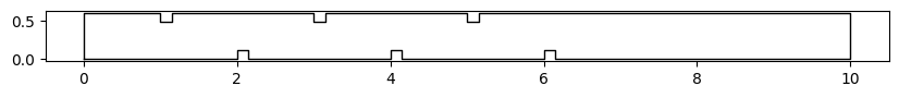
Create a polygon around the domain incorporating the obstacles (add a vertex for all corners of the channel and all corners of the obstacles) by specifying the (x, y) coordinates in the add_vertex function.
[10]:
contour = vector(name='contour') # create the contour vector
contour.add_vertex(wolfvertex(x=origx, y=origy)) # add origin = bottom-left corner
# add obstacles on the lower side
for i in range(n_obs):
x = x_low_obs[i]
y = origy
# add all vertices of the obstacle
contour.add_vertex(wolfvertex(x=x, y=y))
contour.add_vertex(wolfvertex(x=x, y=y + height_obs))
contour.add_vertex(wolfvertex(x=x + width_obs, y=y + height_obs))
contour.add_vertex(wolfvertex(x=x + width_obs, y=y))
# no need to close the obstacle -- just pass to the next one
contour.add_vertex(wolfvertex(x=origx + Lx, y=origy)) # add bottom-right corner
contour.add_vertex(wolfvertex(x=origx + Lx, y=origy + Ly)) # add top-right corner
# add obstacles on the upper side - in reverse order
x_up_obs.reverse() # reverse the list to have the obstacles in the right order
for i in range(n_obs):
x = x_up_obs[i]
y = origy + Ly
# add all vertices of the obstacle
contour.add_vertex(wolfvertex(x=x + width_obs, y=y))
contour.add_vertex(wolfvertex(x=x + width_obs, y=y - height_obs))
contour.add_vertex(wolfvertex(x=x, y=y - height_obs))
contour.add_vertex(wolfvertex(x=x, y=y))
# no need to close the obstacle -- just pass to the next one
contour.add_vertex(wolfvertex(x=origx, y=origy + Ly)) # top-left corner
contour.force_to_close() # force the vector to be closed
Visualize the contour
[11]:
fig, ax = plt.subplots(figsize=(10, 18))
contour.plot_matplotlib(ax)
ax.set_aspect('equal')
Define a magnetic grid, set the contour, and create the mesh
[12]:
# force the vertices to be aligned with the grid
newsim.set_magnetic_grid(dx=dx, dy=dy, origx=origx, origy=origy)
# set the external border of the mesh to be the contour defined above
newsim.set_external_border_vector(contour)
# set the size of the mesh to be dx and dy (in meters)
newsim.set_mesh_fine_size(dx=dx, dy=dy)
# add the block defined by the contour to the mesh
newsim.add_block(contour, dx=dx, dy=dy)
# create the mesh
if newsim.mesh():
print('Meshing done!')
else:
print('Meshing failed!')
# create the fine arrays with prescribed friction coefficient and turbulence
friction_coefficient = 1e-4
newsim.create_fine_arrays(default_frot=friction_coefficient, with_tubulence=True)
newsim.parameters.blocks[0].set_lateral_friction_coefficient(lateral_friction_coefficient=friction_coefficient) # add friction coefficient to the lateral walls
newsim.create_sux_suy() # find the borders where BC can be applied
Meshing done!
Get general information on the mesh
[13]:
print(newsim.get_header())
Shape : 1006 x 66
Resolution : 0.01 x 0.01
Spatial extent :
- Origin : (-0.03 ; -0.03)
- End : (10.030000000000001 ; 0.63)
- Width x Height : 10.06 x 0.66
- Translation : (0.0 ; 0.0)
Null value : 0.0
The origin is not (0.,0.) because the meshing process adds 3 cells around all sides of the domain. This is done to ensure that there is enough space to store neighborhood relationships between blocks in the matrices and to keep at least one fringe hidden all around.
The same information is available with the function get_header_MB, which also returns the number of blocks. In this case, block1 has the correct origin at (0, 0).
[14]:
print(newsim.get_header_MB())
Shape : 1006 x 66
Resolution : 0.01 x 0.01
Spatial extent :
- Origin : (-0.03 ; -0.03)
- End : (10.030000000000001 ; 0.63)
- Width x Height : 10.06 x 0.66
- Translation : (0.0 ; 0.0)
Null value : 0.0
Number of blocks : 1
Block block1 :
Shape : 1006 x 66
Resolution : 0.01 x 0.01
Spatial extent :
- Origin : (0.0 ; 0.0)
- End : (10.06 ; 0.66)
- Width x Height : 10.06 x 0.66
- Translation : (-0.03 ; -0.03)
Null value : 0.0
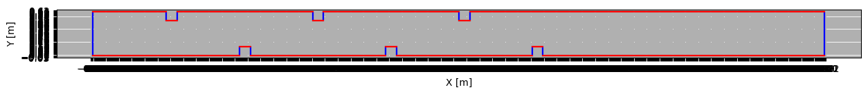
Visualize the topopography
[15]:
fig, ax = newsim.top.plot_matplotlib()
contour.plot_matplotlib(ax)
fig.set_size_inches(15, 3)

Set the simulation parameters
nb_timesteps sets how many timesteps are performed. The writing_frequency and writing_mode keys specify how often the simulation results are saved. Avoid saving results with a large frequency to reduce the file dimension.
Avoid too large CourantNumber (must be \(\leq 1\), preferably \(\leq 0.6\)). However, too small values reduce the timestep, hence increase the computation time.
When visualizing the results, if a checkerboard pattern is observed in the water heights, it very often means that the Courant number is too high. You should then reduce it to avoid this problem.
[16]:
# time parameters
newsim.parameters.set_params_time_iterations(nb_timesteps=100, optimize_timestep=True,
writing_frequency=0.5, writing_mode='Seconds',
initial_cond_reading_mode='Binary',
writing_type='Binary compressed')
# numerical parameters
newsim.parameters.set_params_temporal_scheme(RungeKutta='RK21', CourantNumber=0.35)
# turbulence parameters
newsim.parameters.blocks[0].set_params_turbulence('k-eps HECE', maximum_nut=1e-2) # if needed, increase maximum_nut to avoid numerical issues
newsim.parameters.blocks[0].set_params_surface_friction(model_type='Horizontal and Lateral external borders (Colebrook)') # choose the right function
Print the temporal parameters of the simulation.
[17]:
newsim.parameters.get_params_temporal_scheme()
[17]:
{'RungeKutta': 0.3, 'CourantNumber': 0.35, 'dt_factor': 100.0}
Print the iteration parameters.
[18]:
newsim.parameters.get_params_time_iterations()
[18]:
{'nb_timesteps': 100,
'optimize_timestep': 1,
'first_timestep_duration': 0.1,
'writing_frequency': 0.5,
'writing_mode': 'Seconds',
'writing_type': 'Binary compressed',
'initial_cond_reading_mode': 'Binary',
'writing_force_onlyonestep': 0}
Verify the simulation parameters
Several levels of verbosity are available:
0: Errors only
1: Errors and Warnings
2: Errors, Warnings, and Information
3: Errors, Warnings, Information, and section headers
[19]:
print(newsim.check_all(verbosity=3))
Checking Global Parameters
--------------------------
Time/Iterations
****************
Temporal scheme
****************
Runge-Kutta is valid : 0.3
Courant number is valid : 0.35
dt factor is valid : 100.0
Collapsible building (only global values -- activation depends on the block's param)
********************
Hmax is valid : 0.0
Vmax is valid : 0.0
Qmax is valid : 0.0
Checking Block 1
----------------
Topography operator
*******************
Info : Mean operator
Reconstruction type
********************
Info : Internal reconstruction is constant
Info : Frontier reconstruction is linear with limitation
Info : Free border reconstruction is constant
Info : Number of neighbors for limitation is correct
Info : Limitation of h or h+z is correct
Info : Treatment of frontiers is correct
Flux type
**********
Info : HECE original
Froude max
**********
Info : Froude max is 20.0
Warning : Froude max is high -- Is it useful ?
Conflict resolution
********************
Info : Original conflict resolution
Sediment model
**************
Info : Sediment model not activated
Info : No drifting
Gravity discharge
*****************
Info : Gravity discharge not activated
Steady sediment
****************
Info : Not yet implemented -- Feel free to complete the code -- check_params_steady_sediment
Unsteady topo_bathymetry
***********************
Info : Unsteady topo not activated
Collapse building
*****************
Info : Collapse building not activated
Mobile Contour
**************
Info : Mobile contour not activated
Mobile Forcing
**************
Info : Mobile forcing not activated
Forcing
*******
Info: No forcing
Bridges
*******
Info : Bridges not activated
Info : Bridges file not found
Danger map
*********
Info : Danger map not activated
Turbulence
**********
Info: HECE k-eps model selected
Warning : a too low value of "max_nut" can influence the results -- To be checked by the user in the results
Infiltration
************
Info: No infiltration
Get boundary cells and set boundary conditions
Listing
The list of boundary condition edges can be obtained via list_pot_bc_x and list_pot_bc_y.
The return of these routines consists of a list of 2 Numpy vectors (np.int32). It is therefore quite easy to perform sorting or other actions to select specific edges.
bcx[0]= indices ibcx[1]= indices j
These edges are numbered according to the Fortran convention, i.e., 1-based.
[20]:
bcx = newsim.list_pot_bc_x()
bcy = newsim.list_pot_bc_y()
[21]:
print(f'Potential boundary cells in x direction: {bcx}\n')
print(f'Potential boundary cells in y direction: {bcy}')
Potential boundary cells in x direction: (array([ 4, 4, 4, 4, 4, 4, 4, 4, 4, 4, 4,
4, 4, 4, 4, 4, 4, 4, 4, 4, 4, 4,
4, 4, 4, 4, 4, 4, 4, 4, 4, 4, 4,
4, 4, 4, 4, 4, 4, 4, 4, 4, 4, 4,
4, 4, 4, 4, 4, 4, 4, 4, 4, 4, 4,
4, 4, 4, 4, 4, 104, 104, 104, 104, 104, 104,
104, 104, 104, 104, 104, 104, 119, 119, 119, 119, 119,
119, 119, 119, 119, 119, 119, 119, 204, 204, 204, 204,
204, 204, 204, 204, 204, 204, 204, 204, 219, 219, 219,
219, 219, 219, 219, 219, 219, 219, 219, 219, 304, 304,
304, 304, 304, 304, 304, 304, 304, 304, 304, 304, 319,
319, 319, 319, 319, 319, 319, 319, 319, 319, 319, 319,
404, 404, 404, 404, 404, 404, 404, 404, 404, 404, 404,
404, 419, 419, 419, 419, 419, 419, 419, 419, 419, 419,
419, 419, 504, 504, 504, 504, 504, 504, 504, 504, 504,
504, 504, 504, 519, 519, 519, 519, 519, 519, 519, 519,
519, 519, 519, 519, 604, 604, 604, 604, 604, 604, 604,
604, 604, 604, 604, 604, 619, 619, 619, 619, 619, 619,
619, 619, 619, 619, 619, 619, 1004, 1004, 1004, 1004, 1004,
1004, 1004, 1004, 1004, 1004, 1004, 1004, 1004, 1004, 1004, 1004,
1004, 1004, 1004, 1004, 1004, 1004, 1004, 1004, 1004, 1004, 1004,
1004, 1004, 1004, 1004, 1004, 1004, 1004, 1004, 1004, 1004, 1004,
1004, 1004, 1004, 1004, 1004, 1004, 1004, 1004, 1004, 1004, 1004,
1004, 1004, 1004, 1004, 1004, 1004, 1004, 1004, 1004, 1004, 1004],
dtype=int32), array([ 4, 5, 6, 7, 8, 9, 10, 11, 12, 13, 14, 15, 16, 17, 18, 19, 20,
21, 22, 23, 24, 25, 26, 27, 28, 29, 30, 31, 32, 33, 34, 35, 36, 37,
38, 39, 40, 41, 42, 43, 44, 45, 46, 47, 48, 49, 50, 51, 52, 53, 54,
55, 56, 57, 58, 59, 60, 61, 62, 63, 52, 53, 54, 55, 56, 57, 58, 59,
60, 61, 62, 63, 52, 53, 54, 55, 56, 57, 58, 59, 60, 61, 62, 63, 4,
5, 6, 7, 8, 9, 10, 11, 12, 13, 14, 15, 4, 5, 6, 7, 8, 9,
10, 11, 12, 13, 14, 15, 52, 53, 54, 55, 56, 57, 58, 59, 60, 61, 62,
63, 52, 53, 54, 55, 56, 57, 58, 59, 60, 61, 62, 63, 4, 5, 6, 7,
8, 9, 10, 11, 12, 13, 14, 15, 4, 5, 6, 7, 8, 9, 10, 11, 12,
13, 14, 15, 52, 53, 54, 55, 56, 57, 58, 59, 60, 61, 62, 63, 52, 53,
54, 55, 56, 57, 58, 59, 60, 61, 62, 63, 4, 5, 6, 7, 8, 9, 10,
11, 12, 13, 14, 15, 4, 5, 6, 7, 8, 9, 10, 11, 12, 13, 14, 15,
4, 5, 6, 7, 8, 9, 10, 11, 12, 13, 14, 15, 16, 17, 18, 19, 20,
21, 22, 23, 24, 25, 26, 27, 28, 29, 30, 31, 32, 33, 34, 35, 36, 37,
38, 39, 40, 41, 42, 43, 44, 45, 46, 47, 48, 49, 50, 51, 52, 53, 54,
55, 56, 57, 58, 59, 60, 61, 62, 63], dtype=int32))
Potential boundary cells in y direction: (array([ 4, 4, 5, ..., 1002, 1003, 1003], dtype=int32), array([ 4, 64, 4, ..., 64, 4, 64], dtype=int32))
[22]:
# X borders - 0-based
lmost = int(np.asarray(bcx[0]).min())
rmost = int(np.asarray(bcx[0]).max())
# Y borders - 0-based
ymin = int(np.asarray(bcx[1]).min())
ymax = int(np.asarray(bcx[1]).max())
print(f'Bottom-left cell coordinates: {(lmost, ymin)}')
print(f'Top-right cell coordinates: {(rmost, ymax)}')
Bottom-left cell coordinates: (4, 4)
Top-right cell coordinates: (1004, 63)
Visualize boundary cells (blue for horizontal and red for vertical boundaries).
[ ]:
%matplotlib inline
fig, ax = newsim.plot_borders(xy_or_ij='xy', xcolor='b', ycolor='r')
ax.set_xticks(np.arange(newsim.origx, newsim.endx, newsim.dx))
ax.set_yticks(np.arange(newsim.origy, newsim.endy, newsim.dy))
ax.grid()
fig.set_size_inches(15, 5)
Imposing a Weak Condition
It is possible to impose a weak condition via the add_weak_bc_x and add_weak_bc_y routines.
The following arguments must be specified:
the indices
(i, j)as available in the previous liststhe type of BC
BCType_2D(longitudinal and lateral unit discharge,QXandQY; water level,H)the value (this value does not matter for
NONE, except for99999., which is equivalent to a null value in previous versions)
[25]:
newsim.reset_all_boundary_conditions()
# unit discharge at the leftmost X cells (upstream BC)
for j in range(ymin, ymax+1):
newsim.add_weak_bc_x(i = lmost, j = j, ntype = BCType_2D.QX, value = Qx_ups)
newsim.add_weak_bc_x(i = lmost, j = j, ntype = BCType_2D.QY, value = 0.0) # no lateral flow
# water depth at the rightmost X cells (downstream BC)
for j in range(ymin, ymax+1):
newsim.add_weak_bc_x(i = rmost, j = j, ntype = BCType_2D.H, value = h_dws)
Set initial conditions and other simulation parameters
Initial channel topography
[26]:
top = newsim.read_fine_array('.top') # get a WolfArray object
# create channel elevation row - no need to create a complete 2D array
x = np.arange(0, Lx, dx)
z = - slope * x
[27]:
# copy the channel bed elevation to each row of the top.array
for j in range(ymin, ymax+1):
top.array[lmost:rmost, j] = z
# # if the bed elevation is constant, you can also set the whole array to the same value
# top.array[:,:] = 0.0
print('Topo min : ', top.array.min())
print('Topo max : ', top.array.max())
top.write_all()
Topo min : -0.0
Topo max : -0.0
Initial water depth
[28]:
h = newsim.read_fine_array('.hbin')
# since topography is flat, the water height matrix can be easily edited
h.array[:,:] = h_dws
print('Hauteur min : ', h.array.min())
print('Hauteur max : ', h.array.max())
h.write_all()
Hauteur min : 0.058
Hauteur max : 0.058
Flow rates through X and Y
[29]:
qx = newsim.read_fine_array('.qxbin')
qy = newsim.read_fine_array('.qybin')
qx.array[:,:] = 0.
qy.array[:,:] = 0.
qx.write_all()
qy.write_all()
Friction coefficient
Default law is Manning-Strickler.
[30]:
nManning = newsim.read_fine_array('.frot')
print('Default friction value: ', nManning.array.max())
Default friction value: 1e-04
Final checks and saving simulation
Saving to Disk
Parameters and boundary conditions can be saved to disk in the “.par” file using the save method.
Writing to disk can only be properly performed after defining both the useful parameters and the boundary conditions of the problem.
[31]:
newsim.save()
WARNING:root:No infiltration data to write
You can verify the date of the last modification of the new simulation topography (or any other array).
[32]:
print('Last modified (UTC) : ', newsim.last_modification_date('.top', tz.utc)) # date in UTC
Last modified (UTC) : 2025-05-30 13:06:03.100049+00:00
It is possible to easily read data using read_fine_array or read_MB_array by passing the file extension as an argument.
The ‘.’ in the extension is optional but recommended for better readability.
The return is a WolfArray or WolfArrayMB object (see WolfArray Documentation).
[34]:
# example of reading the napbin matrix
nap = newsim.read_fine_array('.napbin')
nap2 = newsim.read_fine_array('napbin')
print('Comparison of matrix characteristics: ', nap2.is_like(nap))
print('Value comparison: ', np.all(nap2.array.data == nap.array.data))
print('Mask comparison: ', np.all(nap2.array.mask == nap.array.mask))
Comparison of matrix characteristics: True
Value comparison: True
Mask comparison: True
Run the simulation
Once all the files are written to disk, it’s time to start the calculation.
To do so, either run the next cell newsim.run_wolfcli or execute the command wolfcli run_wolf2d_prev genfile=pathtosim in a command window, provided that wolfcli is accessible (e.g., via the PATH).
How to do so:
Open the Windows menu (Windows logo or Ctrl+Esc)
Type
cmdOpen Command Prompt
Type
cd pathtosimType
wolfcli run_wolf2d_prev genfile=pathtosim
pathtosim with the actual directory where this notebook is storedC:\Users\yourname\Desktop\gitlabrepository\simulations).Attention: do not run the cells following the next one before the calculation has finished! Otherwise, the python kernel will crash as the simulation files are being overwritten.
[35]:
newsim.run_wolfcli()
Access the results
If the calculation proceeded as expected, additional files will be present in your simulation directory.
These include:
.RH: results of water height on the calculated meshes (binary - float32).RUH: results of specific discharge along X (binary - float32).RVH: results of specific discharge along Y (binary - float32).RCSR: mesh numbering according to the Compressed Sparse Row standard (binary - int32).HEAD: header containing all position information in the previous files (binary - mixed).RZB: result of bottom elevation (sediment calculation)
Additional files will be present in case of turbulence calculation, depending on the chosen model.
It is recommended to access the results via the Wolfresults_2D class - Wolfresults_2D API.
[94]:
# generate instance of the result object
res = Wolfresults_2D(newsim.filename)
# get number of results
n_res = res.get_nbresults()
print('Number of results: ', res.get_nbresults())
Number of results: 107
You can extract the stored times and the timesteps.
[95]:
# extract time and timesteps
times, timesteps = res.get_times_steps()
print('Times: ', times)
print('Timesteps: ', timesteps)
Times: [ 0. 0.5015121 1.0023386 1.5016546 2.001919 2.5024412
3.0013795 3.5011578 4.0014176 4.502446 5.000809 5.502084
6.001237 6.5023127 7.0011334 7.5017495 8.0009365 8.500862
9.001777 9.501919 10.002204 10.502583 11.001969 11.501813
12.001568 12.502362 13.001185 13.500698 14.000468 14.5026045
15.002597 15.502099 16.001596 16.501358 17.000643 17.50115
18.002254 18.501984 19.000114 19.5023 20.001415 20.5012
21.000227 21.500643 22.001781 22.502323 23.001415 23.501835
24.001543 24.501318 25.001766 25.5022 26.000576 26.502256
27.002222 27.500095 28.002329 28.500319 29.001446 29.501617
30.002073 30.5004 31.001257 31.500914 32.001945 32.50202
33.001144 33.501354 34.000206 34.50019 35.00138 35.50133
36.002228 36.50133 37.00134 37.502007 38.000797 38.50038
39.00075 39.502388 40.00085 40.501328 41.00063 41.50236
42.002472 42.50074 43.000004 43.50125 44.00041 44.50245
45.000984 45.502403 46.000904 46.501858 47.00083 47.501087
48.00019 48.50211 49.001907 49.502216 50.000755 50.500492
51.000793 51.50174 52.00254 52.50011 53.002586 ]
Timesteps: [ 0 157 315 491 671 848 1027 1205 1384 1564 1742 1922
2099 2278 2456 2635 2813 2991 3169 3348 3528 3709 3889 4069
4250 4432 4614 4796 4978 5162 5346 5530 5715 5900 6085 6271
6458 6647 6839 7035 7232 7431 7631 7833 8036 8239 8441 8643
8845 9048 9253 9459 9664 9870 10075 10279 10485 10690 10897 11104
11311 11516 11721 11925 12129 12332 12534 12736 12937 13138 13339 13539
13739 13938 14137 14336 14534 14732 14930 15128 15324 15520 15715 15911
16106 16300 16495 16691 16886 17082 17276 17470 17662 17855 18047 18239
18430 18622 18813 19004 19194 19384 19574 19764 19954 20143 20334]
[96]:
# get result from one specific timestep (0-based)
res.read_oneresult(-1)
The results are stored in the form of blocks, accessible via a dictionary. The key for this dictionary is generated by the getkeyblock function from the wolf_array module, WolfArray API.
Each block contains the results for various unknowns and, if applicable, combined values.
It is possible to choose these combined values via the views_2D Enum - Views_2D API.
The current view of a result object allows to visualize and analyze the defined variable.
[97]:
res.set_current(views_2D.WATERDEPTH) # set the current view to water depth
The matrix of each block can be obtained in three different ways as done in the next cell.
[98]:
fr1 = res[0] # result matrix of block #1 by passing an integer
fr2 = res[getkeyblock(1, addone=False)] # result matrix of block #1 by passing a key generated by getkeyblock
fr3 = res[getkeyblock(0)] # result matrix of block #0 by passing a key generated by getkeyblock
assert fr1 == fr2
assert fr2 == fr3
[99]:
print('Result type: ', type(fr1)) # returned format is of type "WolfArray"
Result type: <class 'wolfhece.wolf_array.WolfArray'>
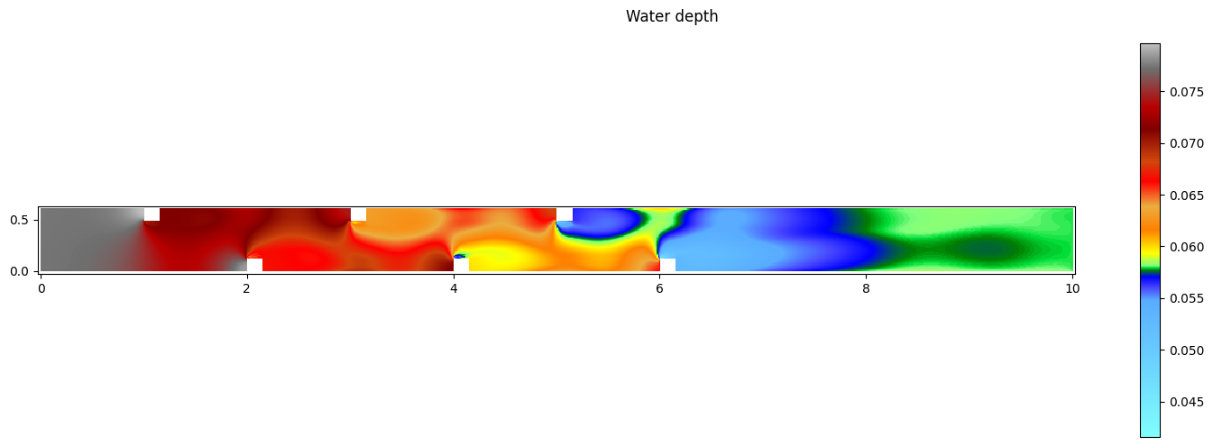
Visualize the results
It is possible to visualize the results of a specific timestep by defining this.
[100]:
ts_result = -1
[101]:
# get the result of the specified timestep
res.read_oneresult(ts_result)
# set current view to the desired variable
res.set_current(views_2D.WATERDEPTH)
print('Minimum water depth: ', res[0].array.min())
print('Maximum water depth: ', res[0].array.max())
fig,ax = res[0].plot_matplotlib()
fig.suptitle('Water depth')
fig.colorbar(ax.images[0], ax=ax)
fig.set_size_inches(15, 5)
fig.tight_layout()
Minimum water depth: 0.041603282
Maximum water depth: 0.07961363
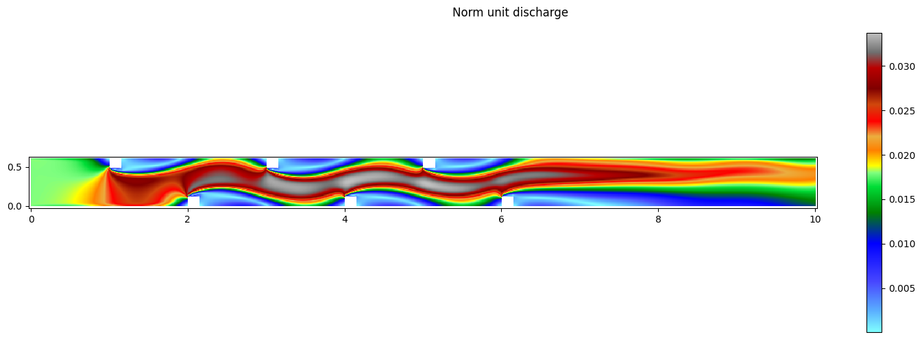
[102]:
res.set_current(views_2D.QNORM)
print('Minimum norm unit discharge:', res[0].array.min())
print('Maximum norm unit discharge:', res[0].array.max())
fig,ax = res[0].plot_matplotlib()
fig.suptitle('Norm unit discharge')
fig.colorbar(ax.images[0], ax=ax)
fig.set_size_inches(15, 5)
fig.tight_layout()
Minimum norm unit discharge: 5.2852378e-05
Maximum norm unit discharge: 0.03371695
[103]:
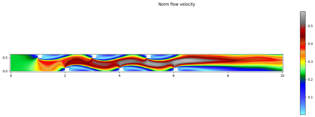
res.set_current(views_2D.UNORM)
print('Minimum norm flow velocity:', res[0].array.min())
print('Maximum norm flow velocity:', res[0].array.max())
fig,ax = res[0].plot_matplotlib()
fig.suptitle('Norm flow velocity')
fig.colorbar(ax.images[0], ax=ax)
fig.set_size_inches(15, 5)
fig.tight_layout()
Minimum norm flow velocity: 0.00089196354
Maximum norm flow velocity: 0.58194137
Generate an animation of the results
Create arrays for the x- and y-axis and ticks for the animation.
[104]:
nbx, nby=int(Lx/dx), int(Ly/dy)
# generate x- and y-axis arrays
x_axis = np.arange(origx, nbx+1, 50)
y_axis = np.arange(origy, nby+1, 30)
# generate x- and y-axis ticks
x_ticks = np.arange(origx, Lx+dx, 0.5)
y_ticks = np.arange(origy, Ly+dy, 0.3)
Get the minimum and maximum velocities to set a constant colorbar for the animation.
[105]:
# get min/max velocities from last time step
res.read_oneresult(-1)
res.set_current(views_2D.UNORM)
u = res[0].array.T
u_min, u_max = u.min(), u.max()
vmin = 0 if u_min >= 0 else u_min
vmax = 0 if u_max < 0 else u_max
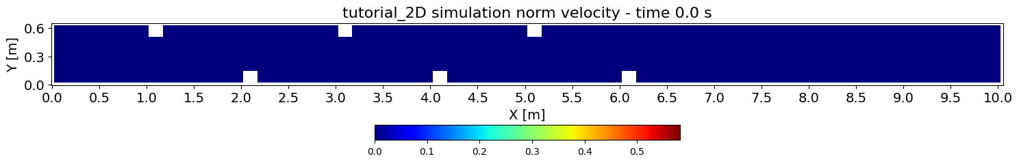
Generate the first frame of the animation (first timestep).
[106]:
%matplotlib inline
# generate animation
init=0 # initial animation timestep
interv=1 # interval between frames
spacing = range(init, n_res, interv) # timesteps to be animated
fig, ax = plt.subplots(figsize=(15, 5))
# first frame setup
res.read_oneresult(spacing[init])
res.set_current(views_2D.UNORM)
im = ax.imshow(res[0].array.T, cmap='jet', interpolation='nearest', vmin=vmin, vmax=vmax)
ax.set_title(f'{simulation_name} simulation norm velocity - time {times[0]} s', fontsize=16)
ax.set_xlabel('X [m]', fontsize=14)
ax.set_ylabel('Y [m]', fontsize=14)
ax.set_xticks(ticks=x_axis, labels=x_ticks, fontsize=14)
ax.set_yticks(ticks=y_axis, labels=y_ticks, fontsize=14)
ax.invert_yaxis()
cbar = fig.colorbar(im, ax=ax, orientation='horizontal', fraction=0.05, pad=0.13)
fig.tight_layout()
Define a function to update the frames of the animation.
Make sure that views_2D. is set to the same variable as the previous cell!
[107]:
def update(time, timestep):
res.read_oneresult(timestep)
res.set_current(views_2D.UNORM)
ax.clear()
im = ax.imshow(res[0].array.T, cmap='jet', interpolation='nearest', vmin=0, vmax=0.45)
title = ax.set_title(f'{simulation_name} simulation norm velocity - time {time} s', fontsize=16)
ax.set_xlabel('X [m]', fontsize=14)
ax.set_ylabel('Y [m]', fontsize=14)
ax.set_xticks(ticks=x_axis, labels=x_ticks, fontsize=14)
ax.set_yticks(ticks=y_axis, labels=y_ticks, fontsize=14)
ax.invert_yaxis() # because WolfArrays are flipped
fig.tight_layout()
return im, title
Generate the animation using the function defined above.
[108]:
%matplotlib inline
ani = animation.FuncAnimation(
fig,
func=lambda i: update(times[i], spacing[i]),
frames=len(spacing),
interval=500, # milliseconds per frame
blit=False # True is not supported with custom plot function
)
d:\ProgrammationGitLab\python3.11\Lib\site-packages\matplotlib\animation.py:908: UserWarning: Animation was deleted without rendering anything. This is most likely not intended. To prevent deletion, assign the Animation to a variable, e.g. `anim`, that exists until you output the Animation using `plt.show()` or `anim.save()`.
warnings.warn(
Save the animation if needed.
Make sure that the variable UNORM is updated if another variable is animated.
[109]:
save_ani = False # set to True to save the animation
if save_ani:
ani.save(f"plots\WOLF_simulations\{simulation_name}_UNORM.mp4",
writer='ffmpeg', dpi=150)
Display the animation in the notbeook.
[110]:
%matplotlib inline
HTML(ani.to_jshtml())
[110]: