Interaction WolfArray/vectors - Rasterizing/Fill in

You can want to rasterize a vector layer to create a raster representation of the vector data. This can be useful for various analyses and visualizations.

To do this, you can use multiple ways.

Importing necessary libraries

# import _add_path # for debugging purposes only - can be removed in production

from wolfhece import is_enough, __version__
assert is_enough("2.2.49"), "Please update wolfhece to 2.2.49 or later - you have " + __version__

from wolfhece.wolf_array import WolfArray, header_wolf, WOLF_ARRAY_FULL_INTEGER, WOLF_ARRAY_FULL_SINGLE
from wolfhece.PyVertexvectors import Zones, zone, vector, wolfvertex as wv
from wolfhece.assets.mesh import Mesh2D

import numpy as np

Creation of an array

First of all, we need to create an array where we will fill in the vector data. The steps are as follows:

1. Create a header

2. Set shape and resolution

3. Create an array from the header

h = header_wolf()
h.shape = (100, 100)
h.set_resolution(1., 1.)

a = WolfArray(srcheader=h)

Creation of a vector

Secondly, we need to create a vector to fill in the array. In this example, we will create a simple polygon (square of 5m x 5m and 1 attached value named ‘testvalue’) with the following steps:

1. Create a vector and add vertices from Numpy array

2. Closed the vector as polygon

3. Add a value to the vector with the key ‘testvalue’

v = vector(fromnumpy= np.asarray([[5.,5.],
                                  [10.,5.],
                                  [10.,10.],
                                  [5.,10.]]))

v.force_to_close() # Close the vector as polygon

v.add_value('testvalue', 5.) # Add an attribute 'testvalue' with value 5.0

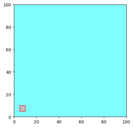
Rasterizing using the attribute value

Finally, we can rasterize the vector into the array using the attribute value ‘testvalue’ to fill in the raster cells that fall within the polygon.

This méthode is a bit like RasterIO.

a.rasterize_vector_valuebyid(v, id= 'testvalue') # Rasterize the vector into the array using the attribute value 'testvalue' to fill in the raster cells that fall within the polygon.

fig, ax = a.plot_matplotlib() # Plot the array using Matplotlib
v.myprop.color = 0xFF0000  # Set the color of the first vector to red with full opacity
v.plot_matplotlib(ax=ax)

(<Figure size 640x480 with 1 Axes>, <Axes: >)

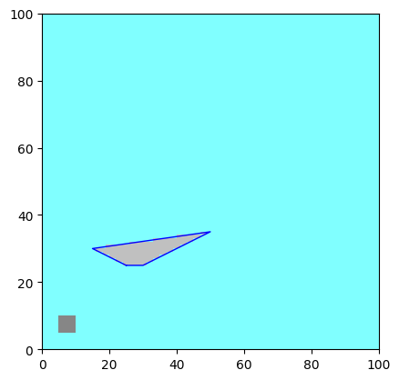
Creation of a zone

In WOLF, a zone is a collection of vectors that can be managed together. Zones allow you to group related vectors for easier manipulation and analysis.

You can create a zone, add vectors to it, and then perform operations on the entire zone as needed.

z = zone()

v2 = vector(fromnumpy= np.asarray([[25.,25.],
                                  [30.,25.],
                                  [50.,35.],
                                  [15.,30.]]))
v2.force_to_close()

z.add_vector(v, forceparent=True)  # Add first vector to the zone and impose the parent attribute of the vector to be the zone
z.add_vector(v2, forceparent=True) # Add second vector to the zone and impose the parent attribute of the vector to be the zone

z.add_values('testvalue', np.asarray([5., 15.])) # Add an attribute 'testvalue' with values 5.0 and 15.0 for each vector in the zone - Values must be ordered as the vectors in the zone

a.rasterize_zone_valuebyid(z, id = 'testvalue') # Rasterize the zone into the array using the attribute value 'testvalue' to fill in the raster cells that fall within the polygons of the vectors in the zone

fig, ax = a.plot_matplotlib() # Plot the array using Matplotlib

v2.myprop.color = 0x0000FF  # Set the color of the second vector to blue with full opacity

v2.plot_matplotlib(ax=ax)

(<Figure size 640x480 with 1 Axes>, <Axes: >)

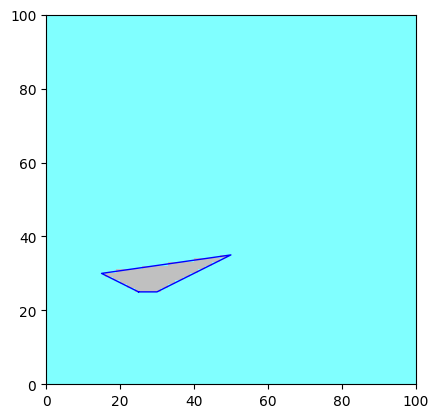
Filling a vector with a scalar value passed by parameter

a.array[:,:] = 1.  # Reset the array to zero
a.fillin_vector_with_value(v2, value=20.)  # Fill in the area of the second vector with the value 20.0

fig, ax = a.plot_matplotlib() # Plot the array using Matplotlib

v2.myprop.color = 0x0000FF  # Set the color of the second vector to blue with full opacity

v2.plot_matplotlib(ax=ax)

(<Figure size 640x480 with 1 Axes>, <Axes: >)

Interpolation “z” values

If the vector has “z” values (elevation or height), you can interpolate these values into the raster array. This is useful for creating digital elevation models (DEMs) or other surface representations from vector data.

Be careful: The interpolation only works if the vector has “z” values assigned to its vertices. If the array is an integer type, the interpolated values will be rounded to the nearest integer by np.ceil().

a.array[:,:] = 1.  # Reset the array to one
v2.z = 20. # Set "z" value of all vertices to 20.0
a.interpolate_on_polygon(v2) # Interpolate the "z" values of the vector into the raster array

fig, ax = a.plot_matplotlib() # Plot the array using Matplotlib
v2.plot_matplotlib(ax=ax)

(<Figure size 640x480 with 1 Axes>, <Axes: >)

Advanced options

When rasterizing or filling in vectors, you can use different methods for determining which raster cells fall within the vector geometry. The available methods are:

• ‘mpl’: Uses Matplotlib’s Path.contains_points method for point-in-polygon testing.

• ‘shapely_strict’: Uses Shapely’s geometry operations for strict point-in-polygon testing.

• ‘shapely_wboundary’: Similar to ‘shapely_strict’, but includes points on the boundary of the polygon.

• ‘rasterio’: Uses Rasterio’s rasterization capabilities.

Shapely methods generally provide better performance and accuracy, especially for complex geometries and large datasets.

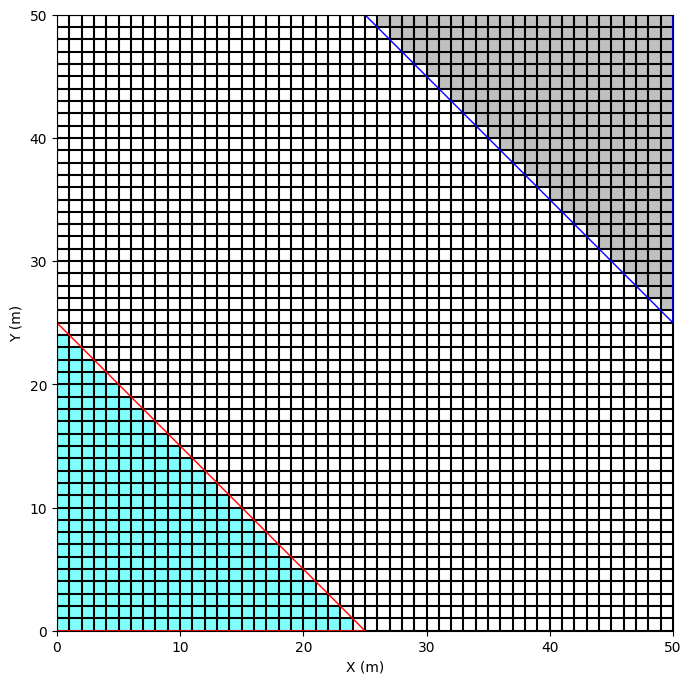
Strictly inside polygon

METHOD = 'shapely_strict'  # Options are: 'mpl', 'shapely_strict', 'shapely_wboundary', 'rasterio'

# Setup of a header and a mesh
header = header_wolf()
xmin_projet = 0
ymin_projet = 0
xmax_projet = 50
ymax_projet = 50

header.set_origin(xmin_projet, ymin_projet)
header.set_resolution(1,1)
header.nbx = xmax_projet - xmin_projet
header.nby = ymax_projet - ymin_projet

mesh = Mesh2D(header) # Useful to plot the cell boundaries

# Setup of the WolfArray
wa = WolfArray(srcheader=header, whichtype=WOLF_ARRAY_FULL_INTEGER)
wa.array[:,:] = 0

# Definition of two vectors
v1 = vector()
v2 = vector()

v1.add_vertex(wv(xmin_projet, ymin_projet, 1))
v1.add_vertex(wv(xmin_projet, (ymin_projet+ymax_projet)/2, 1))
v1.add_vertex(wv((xmin_projet + xmax_projet)/2,ymin_projet, 1))
v1.close_force()

v2.add_vertex(wv((xmin_projet + xmax_projet)/2, ymax_projet, 1))
v2.add_vertex(wv(xmax_projet, (ymin_projet+ymax_projet)/2, 1))
v2.add_vertex(wv(xmax_projet, ymax_projet, 1))
v2.close_force()

# Selection of the cells strictly inside each polygon and setting values in the array
ij = wa.get_ij_inside_polygon(v1, method = METHOD)
wa.array.data[ij[:,0], ij[:,1]] = 1

ij = wa.get_ij_inside_polygon(v2, method = METHOD)
wa.array.data[ij[:,0], ij[:,1]] = 2

fig, ax = wa.plot_matplotlib()
mesh.plot_cells(ax = ax)

v1.myprop.color = 0xFF0000
v2.myprop.color = 0x0000FF

v1.plot_matplotlib(ax=ax)
v2.plot_matplotlib(ax=ax)

fig.set_size_inches(8,8)

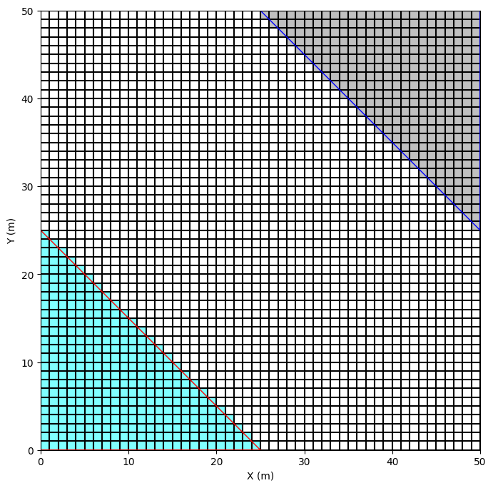
Including boundary points

METHOD = 'shapely_wboundary'  # Options are: 'mpl', 'shapely_strict', 'shapely_wboundary', 'rasterio'

# Setup of a header and a mesh
header = header_wolf()
xmin_projet = 0
ymin_projet = 0
xmax_projet = 50
ymax_projet = 50

header.set_origin(xmin_projet, ymin_projet)
header.set_resolution(1,1)
header.nbx = xmax_projet - xmin_projet
header.nby = ymax_projet - ymin_projet

mesh = Mesh2D(header) # Useful to plot the cell boundaries

# Setup of the WolfArray
wa = WolfArray(srcheader=header, whichtype=WOLF_ARRAY_FULL_INTEGER)
wa.array[:,:] = 0

# Definition of two vectors
v1 = vector()
v2 = vector()

v1.add_vertex(wv(xmin_projet, ymin_projet, 1))
v1.add_vertex(wv(xmin_projet, (ymin_projet+ymax_projet)/2, 1))
v1.add_vertex(wv((xmin_projet + xmax_projet)/2,ymin_projet, 1))
v1.close_force()

v2.add_vertex(wv((xmin_projet + xmax_projet)/2, ymax_projet, 1))
v2.add_vertex(wv(xmax_projet, (ymin_projet+ymax_projet)/2, 1))
v2.add_vertex(wv(xmax_projet, ymax_projet, 1))
v2.close_force()

# Selection of the cells inside each polygon AND on the boundary and setting values in the array
ij = wa.get_ij_inside_polygon(v1, method = METHOD)
wa.array.data[ij[:,0], ij[:,1]] = 1

ij = wa.get_ij_inside_polygon(v2, method = METHOD)
wa.array.data[ij[:,0], ij[:,1]] = 2

fig, ax = wa.plot_matplotlib()
mesh.plot_cells(ax = ax)

v1.myprop.color = 0xFF0000
v2.myprop.color = 0x0000FF

v1.plot_matplotlib(ax=ax)
v2.plot_matplotlib(ax=ax)

fig.set_size_inches(8,8)

Prioritizing vector

When using multiple overlapping or adjacent vectors you can control which vector’s value is used to fill raster cells.

Priority is determined by the order of vectors in the zone or in the provided list; the rasterization follows that sequence. Arrange vectors in the zone/list according to the desired priority.

It is of importance when using methods that may include boundary points, such as ‘shapely_wboundary’, to ensure that the correct vector’s value is applied to cells on shared boundaries.

Important routines

Internally, the main routines used for rasterizing/filling in vectors are:

• get_ij_inside_polygon(): Determines which raster cells fall within a given polygon vector.

• get_xy_inside_polygon(): Similar to get_ij_inside_polygon(), but returns coordinates instead of indices.

• get_xy_infootprint(): Retrieves the coordinates and indices of raster cells that fall within the footprint of a vector.

• get_ij_infootprint(): Similar to get_xy_footprint_vector(), but returns indices instead of coordinates.

print(a.get_ij_inside_polygon.__doc__)

        Return the indices inside a polygon.

        Main principle:
        - First, get all indices in the footprint of the polygon (bounding box + epsilon)
        - Then, test each point if it is inside the polygon with the selected method
        - Filter with the mask if needed

        Returned indices are stored in an array of shape (N,2) with N the number of points found inside the polygon.

        :param myvect: target vector
        :param usemask: limit potential nodes to unmaksed nodes
        :param eps: epsilon for the intersection
        :param method: method to use ('mpl', 'shapely_strict', 'shapely_wboundary', 'rasterio') - default is 'shapely_strict'

print(a.get_xy_inside_polygon.__doc__)

        Return the coordinates inside a polygon.

        Main principle:
        - Get all the coordinates in the footprint of the polygon (taking into account the epsilon if provided)
        - Test each coordinate if it is inside the polygon or not (and along boundary if method allows it)
        - Apply the mask if requested

        Returned values are stored in an array of shape (N,2) with N the number of points found inside the polygon.

        :param myvect: target vector - vector or Shapely Polygon
        :param usemask: limit potential nodes to unmaksed nodes
        :param method: method to use ('mpl', 'shapely_strict', 'shapely_wboundary', 'rasterio') - default is 'shapely_strict'
        :param epsilon: tolerance for the point-in-polygon test - default is 0.

print(a.get_xy_infootprint.__doc__)

        Return the coordinates and the indices of the cells in the footprint of a vector.

        Coordinates are stored in a numpy array of shape (n,2) where n is the number of cells in the footprint.
        Indices are stored in a numpy array of shape (n,2) where n is the number of cells in the footprint. -> See get_ij_infootprint

        Main principle:
        - get the indices with 'get_ij_infootprint'
        - then convert them to coordinates.

        :param myvect: target vector or Shapely Polygon
        :param eps: epsilon to avoid rounding errors
        :return: tuple of two numpy arrays - (coordinates, indices)

print(a.get_ij_infootprint.__doc__)

        Return the indices of the cells in the footprint of a vector

        Main principle:
        - get the bounding box of the vector
        - convert the bounding box to indices
        - limit indices to the array size
        - create a meshgrid of indices

        Indices are stored in a numpy array of shape (n,2) where n is the number of cells in the footprint.

        :param myvect: target vector or Shapely Polygon
        :param eps: epsilon to avoid rounding errors
        :return: numpy array of indices

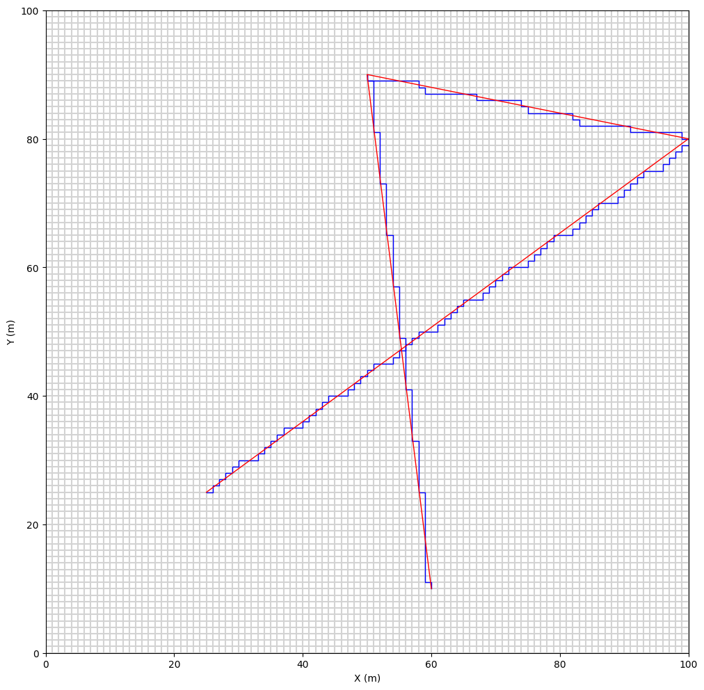
Do not confuse

• rasterize_vector_along_grid : routine of header_wolf class –> rasterize a vector along to the grid - very useful for flow discharge computation bsed on arbitrary cross-sections

• rasterize_vector_valuebyid : routine of WolfArray class –> fill the grid with the value (by its id) inside the polygon formed by the vector

import matplotlib.pyplot as plt
from wolfhece.PyVertex import getRGBfromI, getIfromRGB

v3 = vector(fromnumpy= np.asarray([[25.,25.],
                                  [100.,80.],
                                  [50.,90.],
                                  [60.,10.],
                                  ]))

raster_v3 = a.rasterize_vector_along_grid(v3)

mesh = Mesh2D(a.get_header()) # Asset the mesh for plotting cell boundaries

fig, ax = mesh.plot_cells(color = 'lightgrey')

raster_v3.myprop.color = 0x0000FF # blue using Hex code
raster_v3.plot_matplotlib(ax)

v3.myprop.color = getIfromRGB((255,0,0)) # red using RGB (0-255 scale)
v3.plot_matplotlib(ax)

fig.set_size_inches(12,12)