Creation of a 2D modeling via script
In order to create a 2D simulation, it is necessary to:
Create an instance “prev_sim2d” by going into argument the full access path and the generic name of the simulation
Define a vector/polygon contour delimiting the work area -(optional) Define a “magnetic grid” used to catch vertices of polygons -> allows to align between different models for example.
Define the spatial resolution of the mesh on which the data (topo, rubbing, unknown …) will be provided initially
Define block contours/polygons and their respective spatial resolution
Call the mesher (call to the Fortran code)
Create the mandatory matrices and fill them with the desired values (via script (s) or GUI)
Create the potential edges for boundary conditions (.aux, .suy)
Impose the necessary limits (info: nothing = impermeable)
Configure the problem
Execute the calculation
Treat the results
Import modules
[3]:
from wolfhece.mesh2d.wolf2dprev import prev_sim2D
from wolfhece.PyVertexvectors import zone, Zones, vector, wolfvertex
from wolfhece.wolf_array import WolfArray, WolfArrayMB, header_wolf
from wolfhece.wolfresults_2D import Wolfresults_2D
from wolfhece.mesh2d.cst_2D_boundary_conditions import BCType_2D, Direction, revert_bc_type

from tempfile import TemporaryDirectory
from pathlib import Path
import numpy as np
from datetime import datetime as dt
from datetime import timezone as tz
from datetime import timedelta as td
from typing import Literal, Union
import logging
Definition of the work directory
[4]:
outdir = Path(r'test')
outdir.mkdir(exist_ok=True) # Création du dossier de sortie
print(outdir.name)
test
Verification of the presence of the solver code
Returns the full access path to the code
[5]:
wolfcli = prev_sim2D.check_wolfcli() # méthode de classe, il n'est donc pas nécessaire d'instancier la classe pour l'appeler

if wolfcli:
    print('Code found : ', wolfcli)
else:
    print('Code not found !')
Code found : D:\ProgrammationGitLab\HECEPython\wolfhece\libs\wolfcli.exe
Creation of a 2D simulation object
[ ]:
# Passing the working directory to which we added the generic name of the simulation.
# "Clear" allows you to delete files from the previous simulation.
newsim = prev_sim2D(fname=str(outdir / 'test'), clear=True)

# A "logging.info" message is issued because no file has been found. This is normal!
# If a file is found, it is loaded.
WARNING:root:No infiltration file found
Geometry of the problem
Square domain of total size 1.0 m x 1.0 m.
Definition mode
It is necessary to define an external polygon/outline of the domain to model.
There are six ways of working:
Create a “Vector” object and encode its contact details - via a “Vector” class - see [wolfhece.pyvertexverters] (https://wolf.hece.hece.uliege.be/Autoapi/wolfhece/pyvertexvecotors/index.html)
Define the desired spatial terminals
Define the origin, the size of the mesh and the number of stitches in each direction
Provide a header object
On the basis of an existing matrix - Total grip
On the basis of an existing matrix - outline generated on the basis of its mask
Internally, these 6 procedures will always come back to define a vector contour/polygon, only given accepted by the Fortran code.
Steps of implementation
It is necessary to define an external polygon/outline of the domain to model.
[ ]:
# Magnetic grid - DX and DY are the steps of the grid [m], origx and origy are the coordinates of the first point of the grid.
# The coordinates will be aligned on the magnetic grid by the routine align2grid -- https://wolf.hece.uliege.be/autoapi/wolfhece/wolf_array/index.html#wolfhece.wolf_array.header_wolf.align2grid
newsim.set_magnetic_grid(dx=1., dy=1., origx=0., origy=0.)
# ***** CHOICE *****
# Choisir 1 des 6 options suivantes pour définir le contour externe de la simulation
# ----------------------------------------------------------------------------------
choices = [(1, 'set_external_border_vector'),
(2, 'set_external_border_xy'),
(3, 'set_external_border_nxny'),
(4, 'set_external_border_header'),
(5, 'set_external_border_wolfarray - mode emprise'),
(6, 'set_external_border_wolfarray - mode contour')]
choice = 1
if choice not in [c[0] for c in choices]:
logging.error('Invalid choice !')
elif choice == 1:
# Define the extrenal contour
extern = vector()
extern.add_vertex(wolfvertex(0., 0.))
extern.add_vertex(wolfvertex(1., 0.))
extern.add_vertex(wolfvertex(1., 1.))
extern.add_vertex(wolfvertex(0., 1.))
extern.close_force()
print('Nombre de vertices : ', extern.nbvertices)
print('5 vertices car la polygone est fermé et le dernier point est aux mêmes coordonnées que le premier.')
# Transfert du polygone comme contour externe de simulation.
# Le contour externe est la limite de maillage.
# Ensemble, les polygones de blocs doivent entourer complètement le contour externe.
newsim.set_external_border_vector(extern)
elif choice == 2:
# via des bornes
newsim.set_external_border_xy(xmin= 0., xmax= 1., ymin= 0., ymax= 1.)
elif choice == 3:
# encore via une description de la matrice
# ATTENTION : ici dx et dy ne sont pas nécessairement les mêmes que ceux du maillage fin.
newsim.set_external_border_nxny(xmin= 0, ymin=0., nbx= 10, nby= 10, dx= 0.1, dy= 0.1)
elif choice == 4:
# Ici rien de bien intéressant vis-à-vis du choix précédent mais il est possible
# d'obtenir un header depuis n'importe quelle matrice
header = header_wolf()
header.origx = 0.
header.origy = 0.
header.dx = 0.1
header.dy = 0.1
header.nbx = 10
header.nby = 10
newsim.set_external_border_header(header)
elif choice == 5:
# On peut aussi choisir de définir le contour externe à partir
# d'une matrice de donnée de type WolfArray
# Mode emprise/header
# Comme on n'a pas de données chargées, on crée une matrice de toute pièce.
header = header_wolf()
header.origx = 0.
header.origy = 0.
header.dx = 1.
header.dy = 1.
header.nbx = 1
header.nby = 1
src_array = WolfArray(srcheader=header)
newsim.set_external_border_wolfarray(src_array, mode='header', abs=True)
# L'emprise n'a pas besoin que la matrice soit masquée, mais c'est possible.
# Dans ce dernier cas, le masque est ignoré lors de la création de l'emprise.
elif choice == 6:
# On peut aussi choisir de définir le contour externe à partir
# d'une matrice de données de type WolfArray
# Mode contour/masque
# Comme on n'a pas de données chargées, on crée une matrice de toute pièce.
#
# ATTENTIOn : la recherche d'un contour demande que la matrice soit bornée par des valeurs masquées.
header = header_wolf()
header.origx = -1.
header.origy = -1.
header.dx = 1.
header.dy = 1.
header.nbx = 3
header.nby = 3
src_array = WolfArray(srcheader=header)
# complete way
src_array.array[0,:] = 0.
src_array.array[-1,:] = 0.
src_array.array[:,0] = 0.
src_array.array[:,-1] = 0.
src_array.mask_data(src_array.nullvalue)
# or more simply
#src_array.nullify_border(width=1)
newsim.set_external_border_wolfarray(src_array, mode='contour', abs=True)
# ***** End of choice *****
# By default, the polygon coordinates will be translated for the point (Xmin, Ymin) or in (0, 0).
# Translation info in the '.trl' file
# To avoid translation, we can modify the property "translate_origin2zero".
newsim.translate_origin2zero = True
# Choice of fine mesh spatial steps [M].
newsim.set_mesh_fine_size(dx=0.1, dy=0.1)
# Addition of a block with its specific space step [M].
# We can define a particular outline or reuse the external outline.
extern = newsim.external_border
newsim.add_block(extern, dx=0.2, dy=0.2)
# (optional) Addition of other blocks ...
# Meal of the problem
# - Creation of a file without extension (empty) - Useful for retrocompatibility with the previous versions of Wolf.
# - Writing on disk of the mesh description file (. Block)
# - Calculation of the "fine" grip (can only be done once all the blocks defined because depends on the maximum spatial resolution of the blocks)
# - Call for Fortran code (mesh phase only) - wolfcli must be defined - command "Run_wolf2d_Prev" with argument "Genfile = '/path/to/file'"
# - The Fortran will create the files:
# - ".Mnap" Block mesh and relationships between blocks
# - ".nfo" Screen outputs from the Fortran code
# - ".xy" external outline of the mesh (for graphical interface)
# - ".blx" and ". Bly" free edges of the MB mesh (useful only for Fortran developers)
# - ".cmd" Interaction file with Fortran code under calculation
# - Creation of the file ".napbin" by the Python code (fine grip on which the data must be provided) - will serve as "mask" for data matrices
if newsim.mesh():
print('Meshing done !')
else:
print('Meshing failed !')
# Creation of Data Matrices - Fine grip - Binary format [NP.FLOAT32] - Shape (NBX, NBY)
# - ".top" Topography file [m]
# - ".hbin" Initial water height condition [m]
# - ".Qxbin" Initial specific debit condition according to x [m²/s]
# - ".Qybin" Initial condition of specific flow according to Y [m²/s]
# - ".frot" friction coefficient (default law: manning - "n" units [s/m^(1/3) - reverse of the 'K' de Strickler]) - Default value: 0.04
# - ".Inf" infiltration zoning - not to be confused with the ".fil" file which will contain the values of infiltration flow rates [m³/s]
# If "with_Tubulence" is true, the files ".kbin" and ".pops" will be created in addition and will contain turbulent kinetic energy.
newsim.create_fine_arrays(default_frot=0.04, with_tubulence=False)
# Research on the edges with potential limits on the basis of the matrix ".napbin" and writing of files ".sux" and ".suy"
# - Research mode: edge separating a masked value of an unseated value - Succesive clogging according to x and y
# -".Sux" enumeration of the clues [i, j] of the fine mesh located on the right of an edge oriented according to Y -> [i, j] relating to the edge [I -1/2, j]
#-".Suy" list of clues [i, j] of the fine mesh located above an edge oriented according to x-> [i, j] relating to the edge [i, j-1/2]
newsim.create_sux_suy()
Nombre de vertices :  5
5 vertices car la polygone est fermé et le dernier point est aux mêmes coordonnées que le premier.
Meshing done !
Summary of the spatial grip
It is possible to display information from the fine or MB mesh via “Get_header” and/or “Get_header_mb”
In this specific case, shape == (18, 18) because the fine mesh is resolved (0.1, 0.1) and the maximum block size is (0.2, 0.2)
Or (10x10) for the square domain of (1.0, 1.0) to a resolution of (0.1, 0.1) to which we add a fringe corresponding to (dx_max + 2 * dx_fin) on either side.
This fringe is necessary to ensure that there is enough space to store the neighborhood relationships between blocks in the matrices and to keep at least one masked fringe all around.
So (10 + 2 * (0.2 + 2 * 0.1) / 0.1, 10 + 2 * (0.2 + 2 * 0.1) / 0.1) = (18, 18)
The fringe width is also which explains the values of the origin (-0.4, -0.4). This in order to keep (0.0, 0.0) to (xmin, ymin) of the mesh outdoor polygon.
[8]:
print(newsim.get_header())
Shape  : 18 x 18
Resolution  : 0.1 x 0.1
Spatial extent :
   - Origin : (-0.4 ; -0.4)
   - End : (1.4 ; 1.4)
   - Widht x Height : 1.8 x 1.8
   - Translation : (0.0 ; 0.0)
Null value : 0.0
The same type of information is available in MB.
[9]:
print(newsim.get_header_MB())
Shape  : 18 x 18
Resolution  : 0.1 x 0.1
Spatial extent :
   - Origin : (-0.4 ; -0.4)
   - End : (1.4 ; 1.4)
   - Widht x Height : 1.8 x 1.8
   - Translation : (0.0 ; 0.0)
Null value : 0.0

Number of blocks : 1

Block block1 :

Shape  : 11 x 11
Resolution  : 0.2 x 0.2
Spatial extent :
   - Origin : (-0.19999999999999996 ; -0.19999999999999996)
   - End : (2.0 ; 2.0)
   - Widht x Height : 2.2 x 2.2
   - Translation : (-0.4 ; -0.4)
Null value : 0.0
A little help on the files, their content and the type of storage
[10]:
print(newsim.help_files())
Text files
----------
Infiltration hydrographs [m³/s] : .fil
Resulting mesh [-] : .mnap
Translation to real world [m] : .trl


Fine array - monoblock
----------------------
Mask [-] : .napbin [int16]
Bed Elevation [m] : .top [float32]
Bed Elevation - computed [m] : .topini_fine [float32]
Roughness coefficient [law dependent] : .frot [float32]
Infiltration zone [-] : .inf [int32]
Initial water depth [m] : .hbin [float32]
Initial discharge along X [m^2/s] : .qxbin [float32]
Initial discharge along Y [m^2/s] : .qybin [float32]
Rate of dissipation [m²/s³] : .epsbin [float32]
Turbulent kinetic energy [m²/s²] : .kbin [float32]
Z level under the deck of the bridge [m] : .bridge [float32]


Multiblock arrays
-----------------
MB - Bed elevation [m] : .topini [float32]
MB - Water depth [m] : .hbinb [float32]
MB - Discharge X [m²/s] : .qxbinb [float32]
MB - Discharge Y [m²/s] : .qybinb [float32]
MB - Roughness coeff : .frotini [float32]
MB - Rate of dissipation [m²/s³] : .epsbinb [float32]
MB - Turbulent kinetic energy [m²/s²] : .kbinb [float32]
Setting
When initializing the simulation, default parameter values are defined. They are identical to those imposed by the VB6 code (for retrocompatibility).
These values are commonly used to obtain a stationary state in pure water. The default temporal diagram is a Runge -Kutta 21 - weights (0.7; 0.3).
All settings are of course customizable by the user.
In an attempt to simplify access to values, they are separated between “active” values and “default” values.
When active values are accessed, the returned dictionary only contains the parameters whose value differs from default values.
This does not mean that the values of other parameters are 0
The parameters are split into 2 main categories:
global simulation parameters (shared by all blocks)
specific block parameters
In the VB6 interface, a separation is made in “general” and “debug” parameter. This distinction does not exist more facial in python even if the organization of files is in no way changed.
It will therefore always be possible to operate the VB6 and/or Python interface for the same simulation.
Groups
The different parameters are grouped by theme.
It is possible to obtain the name of these groups via “Get_parameters_Groups”
[ ]:
groups = newsim.get_parameters_groups() # List of parameter groups - Str - sorted in alphabetical order

print('Number of parameter groups: ', len(groups))

# First letter display

for letter in 'abcdefghijklmnopqrstuvwxyz':

    group = [g for g in groups if g[0].lower() == letter]

    if group:
        print(f'Groupe {letter.upper()} : {len(group)}', group)
Nombre de groupes de paramètres :  34
Groupe B : 3 ['Boundary conditions', 'Bridge', 'Buildings']
Groupe C : 2 ['Collapsible buildings', 'Computation domain']
Groupe D : 2 ['Danger map', 'Duration of simulation']
Groupe F : 3 ['Forcing', 'Friction', 'Frictional fluid']
Groupe G : 1 ['Geometry']
Groupe I : 5 ['Infiltration', 'Infiltration weir poly3', 'Infiltration weirs', 'Initial condition', 'Initial conditions']
Groupe M : 3 ['Mesher', 'Mobile contour', 'Mobile forcing']
Groupe N : 1 ['Numerical options']
Groupe O : 1 ['Options']
Groupe P : 1 ['Problem']
Groupe R : 2 ['Reconstruction', 'Results']
Groupe S : 4 ['Sediment', 'Spatial scheme', 'Splitting', 'Stopping criteria']
Groupe T : 2 ['Temporal scheme', 'Turbulence']
Groupe U : 1 ['Unsteady topo-bathymetry']
Groupe V : 3 ['VAM5 - Turbulence', 'Variable infiltration', 'Variable infiltration 2']
Settings
The set of parameters can be obtained via “Get_parameters_Groups_and_names” which returns a list of TUPLES (Group, Param).
It is also possible to list the parameters of a group via “get_parameters_in_group”.
The values of the parameters are numeric (int or float). However, it is possible, via Gui, to choose the configuration via more explicit keywords.
Aid on the parameters can also be obtained via “help_parameter” and/or “help_values_parameter”. The aid is present in the form of a short and potentially long/explicit chain. The first value returned by the “help_parameter” function indicates whether the scope is global or on a block.
[ ]:
all_params = newsim.get_parameters_groups_and_names() # List of parameter groups and parameters - sorted in alphabetical order

print(all_params)
[('Boundary conditions', 'Nb strong BC (not editable)'), ('Boundary conditions', 'Nb weak BC X (not editable)'), ('Boundary conditions', 'Nb weak BC Y (not editable)'), ('Boundary conditions', 'Unsteady BC'), ('Bridge', 'Activate'), ('Buildings', 'Collapsable'), ('Collapsible buildings', 'H max'), ('Collapsible buildings', 'V max'), ('Collapsible buildings', 'Q max'), ('Computation domain', 'Using tags'), ('Computation domain', 'Strip width for extension'), ('Computation domain', 'Delete unconnected cells every'), ('Danger map', 'Compute'), ('Danger map', 'Minimal water depth'), ('Duration of simulation', 'Total steps'), ('Duration of simulation', 'Time step'), ('Forcing', 'Activate'), ('Friction', 'Global friction coefficient'), ('Friction', 'Lateral Manning coefficient'), ('Friction', 'Surface computation method'), ('Frictional fluid', 'Density of the fluid'), ('Frictional fluid', 'Saturated height'), ('Frictional fluid', 'Consolidation coefficient'), ('Frictional fluid', 'Interstitial pressure (t=0)'), ('Geometry', 'Dx'), ('Geometry', 'Dy'), ('Geometry', 'Nx'), ('Geometry', 'Ny'), ('Geometry', 'Origin X'), ('Geometry', 'Origin Y'), ('Infiltration', 'Forced correction ux'), ('Infiltration', 'Forced correction vy'), ('Infiltration weir poly3', 'a'), ('Infiltration weir poly3', 'b'), ('Infiltration weir poly3', 'c'), ('Infiltration weir poly3', 'd'), ('Infiltration weirs', 'Cd'), ('Infiltration weirs', 'Z'), ('Infiltration weirs', 'L'), ('Initial condition', 'To egalize'), ('Initial condition', 'Water level to egalize'), ('Initial conditions', 'Reading mode'), ('Mesher', 'Mesh only'), ('Mesher', 'Remeshing mode'), ('Mesher', 'Number of blocks (not editable)'), ('Mobile contour', 'Active'), ('Mobile forcing', 'Activate'), ('Numerical options', 'Water depth min for division'), ('Numerical options', 'Water depth min'), ('Numerical options', 'Water depth min to compute'), ('Numerical options', 'Exponent Q null on borders'), ('Numerical options', 'Reconstruction slope mode'), ('Numerical options', 'H computation mode (deprecated)'), ('Numerical options', 'Latitude position'), ('Numerical options', 'Troncature (deprecated)'), ('Numerical options', 'Smoothing mode (deprecated)'), ('Options', 'Topography'), ('Options', 'Friction slope'), ('Options', 'Modified infiltration'), ('Options', 'Reference water level for infiltration'), ('Options', 'Inclined axes'), ('Options', 'Variable topography'), ('Problem', 'Number of unknowns'), ('Problem', 'Number of equations'), ('Problem', 'Unequal speed distribution'), ('Problem', 'Conflict resolution'), ('Problem', 'Fixed/Evolutive domain'), ('Reconstruction', 'Reconstruction method'), ('Reconstruction', 'Interblocks reconstruction method'), ('Reconstruction', 'Free border reconstruction method'), ('Reconstruction', 'Number of neighbors'), ('Reconstruction', 'Limit water depth or water level'), ('Reconstruction', 'Frontier'), ('Reconstruction', 'Froude maximum'), ('Results', 'Writing interval'), ('Results', 'Writing interval mode'), ('Results', 'Writing mode'), ('Results', 'Only one result'), ('Sediment', 'Porosity'), ('Sediment', 'Mean diameter'), ('Sediment', 'Relative density'), ('Sediment', 'Theta critical velocity'), ('Sediment', 'Drifting model'), ('Sediment', 'Convergence criteria - bottom'), ('Sediment', 'Convergence criteria - sediment'), ('Sediment', 'Model type'), ('Sediment', 'Active infiltration'), ('Sediment', 'Write topography'), ('Sediment', 'Hmin for computation'), ('Sediment', 'With gravity discharge'), ('Sediment', 'Critical slope'), ('Sediment', 'Natural slope'), ('Sediment', 'Reduction slope'), ('Sediment', 'D30'), ('Sediment', 'D90'), ('Spatial scheme', 'Limiter type'), ('Spatial scheme', 'Venkatakrishnan k'), ('Spatial scheme', 'Wetting-Drying mode'), ('Spatial scheme', 'Non-erodible area'), ('Splitting', 'Splitting type'), ('Stopping criteria', 'Stop computation on'), ('Stopping criteria', 'Epsilon'), ('Temporal scheme', 'Runge-Kutta'), ('Temporal scheme', 'Courant number'), ('Temporal scheme', 'Factor for verification'), ('Temporal scheme', 'Optimized time step'), ('Temporal scheme', 'Mac Cormack (deprecated)'), ('Temporal scheme', 'Local time step factor'), ('Turbulence', 'Model type'), ('Turbulence', 'alpha coefficient'), ('Turbulence', 'Kinematic viscosity'), ('Turbulence', 'Maximum value of the turbulent viscosity'), ('Turbulence', 'C3E coefficient'), ('Turbulence', 'CLK coefficient'), ('Turbulence', 'CLE coefficient'), ('Unsteady topo-bathymetry', 'Model type'), ('VAM5 - Turbulence', 'Vertical viscosity'), ('VAM5 - Turbulence', 'Model type'), ('Variable infiltration', 'a'), ('Variable infiltration', 'b'), ('Variable infiltration', 'c'), ('Variable infiltration 2', 'd'), ('Variable infiltration 2', 'e')]
[ ]:
params = newsim.get_parameters_in_group('Friction') # List of group 'friction' parameters

print(params)
['Global friction coefficient', 'Lateral Manning coefficient', 'Surface computation method']
Examples of help on:
A block parameter
A global parameter
[14]:
target, comment, full_comment = newsim.help_parameter('problem', 'Number of unknowns')

print('Global or Block : ', target)
print('Aide courte :\t', comment)
print('Aide complète :\t', full_comment)

print()

target, comment, full_comment = newsim.help_parameter('duration', 'total steps')

print('Global or Block : ', target)
print('Aide courte :\t', comment)
print('Aide complète :\t', full_comment)
ERROR:root:Group duration or parameter total steps not found
Global or Block :  Block
Aide courte :    Number of unknowns (integer) - default = 4
Aide complète :  If a turbulence model is selected, the number of unknowns will be increased by the computation code accordingly to the number of additional equations

Global or Block :  -
Aide courte :    -
Aide complète :  -
[15]:
vals = newsim.help_values_parameter('friction', 'Surface computation method')

if vals is not None:
    print('Valeurs possibles : \n')
    for key, vals in vals.items():
        print(key, vals)
Valeurs possibles :

Horizontal 0
Modified surface corrected 2D (HECE) 6
Modified surface corrected 2D + Lateral external borders (HECE) 7
Horizontal and Lateral external borders 1
Modified surface (slope) 2
Modified surface (slope) + Lateral external borders 3
Horizontal and Lateral external borders (HECE) 4
Modified surface (slope) + Lateral external borders (HECE) 5
Horizontal -- Bathurst -2
Horizontal -- Bathurst-Colebrook -5
Horizontal -- Chezy -1
Horizontal -- Colebrook -3
Horizontal -- Barr -4
Horizontal -- Bingham -6
Horizontal -- Frictional fluid -61
Horizontal and Lateral external borders (Colebrook) -34
Horizontal and Lateral external borders (Barr) -44
Tolerance to the failure of breakage
A certain tolerance is authorized in writing groups and parameters.
A function “sanitize_group_name” allows you to try to find the information encoded.
It is recommended to use it to check your script.
[ ]:
# OK
print('This example will work because only a breakage error is corrected.\n')

group1, name1 = newsim.sanitize_group_name('fricTION', 'SurFAce computation methOD')

assert group1 == 'Friction'
assert name1 == 'Surface computation method'

print('Group : ', group1)
print('Name : ', name1)

# KO
print('\nThis example will not work because a striking error is present in the group.\n')

group2, name2 = newsim.sanitize_group_name('friTION', 'SurFAce computation methOD')

assert group2 is None
assert name2 == 'Surface computation method'

print('Group : ', group2)
print('Name : ', name2)
ERROR:root:Group friTION or parameter SurFAce computation methOD not found
Cet exemple va fonctionner car seule une erreur de casses est corrigée.

Group :  Friction
Name :  Surface computation method

Cet exemple ne va pas fonctionner car une erreur de frappe est présente dans le groupe.

Group :  None
Name :  Surface computation method
List of active settings
[ ]:
# Recovery of a dictionnaiore with all the active parameters of the simulation, that is to say those which are different from the default values
newsim.get_active_parameters_extended() # -- Extended to also obtain all block settings
{'Geometry': {'Dx': 0.1,
  'Dy': 0.1,
  'Nx': 18,
  'Ny': 18,
  'Origin X': -0.4,
  'Origin Y': -0.4},
 'Block 0': {}}
List of all settings
[ ]:
all = newsim.get_all_parameters()

print('Number of parameter groups : ', len(all))
print('Number of parameters : ', sum([len(p) for p in all.values()]))
Nombre de groupes de paramètres :  11
Nombre de paramètres :  57
Imposing a parameter
The modification of the value of an individual parameter can be done via “set_parameter” which takes as arguments:
The name of the group
The name of the parameter
The value (int or float) -The block index (1-based) if it is a block parameter-a value of -1 or ‘all’ will impose the same parameter value on all current blocks present in the simulation
[19]:
group, name = newsim.sanitize_group_name('friction', 'Surface computation method')
newsim.set_parameter(group, name, value = 3, block = 1)

active = newsim.get_active_parameters_block(1) # dictionnaire des paramètres actifs du bloc 1

if group not in active:
    print('Le groupe n\'est pas dans les paramètres actifs.')
else:
    if name not in active[group]:
        print('Le groupe existe mais Le paramètre a sa valeur par défaut')
    else:
        print(active[group][name])

print('--')

all    = newsim.get_all_parameters_block(1)    # dictionnaire de tous les paramètres du bloc 1

print('Tous les paramètres :')
print(all[group][name])
3
--
Tous les paramètres :
3
For regulars of the VB6 code, specialists and nostalgic, it is also possible to work on the basis of lists of “general” and “debug” parameters.
To do this, you must use “Get_parameters_from_List” and “Set_parameters_from_list”.
[ ]:
glob_gen = newsim.get_parameters_from_list('Global', 'General')
glob_dbg = newsim.get_parameters_from_list('Global', 'Debug')

print('Number of global/general parameters: ', len(glob_gen))
print('Number of global parameters/debug: ', len(glob_dbg))

block_gen = newsim.get_parameters_from_list('Block', 'General', 1)
block_dbg = newsim.get_parameters_from_list('Block', 'Debug', 1)

print('Number of block/general parameters: ', len(block_gen))
print('Number of Block/Debug settings: ', len(block_dbg))
Nombre de paramètres Globaux/Généraux:  36
Nombre de paramètres Globaux/Debug:  60
Nombre de paramètres de Bloc/Généraux:  23
Nombre de paramètres de Bloc/Debug:  60
The association with group names and parameters is obtained via “Get_Group_Name_from_List”.
[21]:
glob_gen_key = newsim.get_group_name_from_list('Global', 'General')
glob_dbg_ket = newsim.get_group_name_from_list('Global', 'Debug')
block_gen_key = newsim.get_group_name_from_list('Block', 'General')
block_dbg_key = newsim.get_group_name_from_list('Block', 'Debug')

def print_group_param(target:Literal['Global', 'Block'],
                      which:Literal['General', 'Debug'],
                      idx:int):

    if target == 'Global':
        if which == 'General':
            print(f'Groupe "{glob_gen_key[idx-1][0]}" : Param "{glob_gen_key[idx-1][1]}"')
        else:
            print(f'Groupe "{glob_dbg_ket[idx-1][0]}" : Param "{glob_dbg_ket[idx-1][1]}"')
    else:
        if which == 'General':
            print(f'Groupe "{block_gen_key[idx-1][0]}" : Param "{block_gen_key[idx-1][1]}"')
        else:
            print(f'Groupe "{block_dbg_key[idx-1][0]}" : Param "{block_dbg_key[idx-1][1]}"')

print_group_param('Global', 'General', 1)
Groupe "Duration of simulation" : Param "Total steps"
Typage of the settings
The parameters are whole or floating.
The expected type is specified in the help/comment associated with each paameter.
During the imposition of value, a conversion is forced into the right type.
If an error occurs, first check your code before shouting at WOLF. ;-)
Settings (very) frequently used/defined
A list of the most frequent parameters are available via “Get_Frequent_parameters”.
[22]:
print(newsim.get_frequent_parameters.__doc__)

freq_glob, freq_block, (idx_glog_gen, idx_glob_dbg, idx_bl_gen, idx_bl_dbg) = newsim.get_frequent_parameters()

print('Paramètres globaux/généraux fréquents : ', freq_glob)
print('Paramètres de bloc fréquents : ', freq_block)
        Renvoi des paramètres de simulation fréquents

        Les valeurs retournées sont :
            - les groupes et noms des paramètres globaux
            - les groupes et noms des paramètres de blocs
            - les indices des paramètres globaux (generaux et debug) et de blocs (generaux et debug)


Paramètres globaux/généraux fréquents :  [('Duration of simulation', 'Total steps'), ('Results', 'Writing interval'), ('Results', 'Writing interval mode'), ('Initial conditions', 'Reading mode'), ('Temporal scheme', 'Runge-Kutta'), ('Temporal scheme', 'Courant number'), ('Spatial scheme', 'Wetting-Drying mode'), ('Computation domain', 'Delete unconnected cells every')]
Paramètres de bloc fréquents :  [('Reconstruction', 'Froude maximum'), ('Problem', 'Conflict resolution'), ('Problem', 'Fixed/Evolutive domain'), ('Options', 'Friction slope'), ('Options', 'Modified infiltration'), ('Options', 'Reference water level for infiltration'), ('Turbulence', 'Model type'), ('Turbulence', 'alpha coefficient'), ('Turbulence', 'Kinematic viscosity'), ('Not used', '4'), ('Variable infiltration', 'a'), ('Variable infiltration', 'b'), ('Variable infiltration', 'c'), ('Friction', 'Lateral Manning coefficient'), ('Friction', 'Surface computation method'), ('Danger map', 'Compute'), ('Danger map', 'Minimal water depth'), ('Bridge', 'Activate'), ('Infiltration weirs', 'Cd'), ('Infiltration weirs', 'Z'), ('Variable infiltration 2', 'd'), ('Variable infiltration 2', 'e'), ('Infiltration weirs', 'L'), ('Turbulence', 'Maximum value of the turbulent viscosity'), ('Infiltration weir poly3', 'a'), ('Infiltration weir poly3', 'b'), ('Infiltration weir poly3', 'c'), ('Infiltration weir poly3', 'd'), ('Turbulence', 'C3E coefficient'), ('Turbulence', 'CLK coefficient'), ('Turbulence', 'CLE coefficient')]
To look more …
[23]:
print(newsim.help_useful_fct.__doc__)
print(newsim.help_useful_fct()[0])
        Useful functions/routines for parameters manipulation

        :return (ret, dict) : ret is a string with the description of the function, dict is a dictionary with the function names sorted by category (Global, Block) and type (set, get, reset, check)


Useful functions can be found to set, get, reset and check parameters.

Here is a list of implemented functions :

Setter in global parameters
***************************

    set_params_geometry
    set_params_time_iterations
    set_params_temporal_scheme
    set_params_collapsible_building

Getter in global parameters
***************************

    get_params_time_iterations
    get_params_temporal_scheme
    get_params_collapsible_building

Setter in block parameters
**************************

    set_params_topography_operator
    set_params_reconstruction_type
    set_params_flux_type
    set_params_froud_max
    set_params_conflict_resolution
    set_params_sediment
    set_params_gravity_discharge
    set_params_steady_sediment
    set_params_unsteady_topo_bathymetry
    set_params_collapse_building
    set_params_mobile_contour
    set_params_mobile_forcing
    set_params_bridges
    set_params_danger_map
    set_params_surface_friction
    set_params_turbulence
    set_params_vam5_turbulence
    set_params_infiltration_momentum_correction
    set_params_infiltration_bridge
    set_params_infiltration_weir
    set_params_infiltration_weir_poly3
    set_params_infiltration_polynomial2
    set_params_infiltration_power
    set_params_bingham_model
    set_params_frictional_model

Getter in block parameters

**************************

    get_params_topography_operator
    get_params_reconstruction_type
    get_params_flux_type
    get_params_froud_max
    get_params_conflict_resolution
    get_params_sediment
    get_params_gravity_discharge
    get_params_steady_sediment
    get_params_unsteady_topo_bathymetry
    get_params_collapse_building
    get_params_mobile_contour
    get_params_bridges
    get_params_danger_maps
    get_params_surface_friction
    get_params_turbulence
    get_params_vam5_turbulence
    get_params_infiltration
    get_params_infiltration_momentum_correction
    get_params_frictional

Resetter in global parameters

*****************************

    reset_params_time_iterations
    reset_params_temporal_scheme

Resetter in block parameters

****************************

    reset_params_topography_operator
    reset_params_reconstruction_type
    reset_params_flux_type
    reset_params_froud_max
    reset_params_conflict_resolution
    reset_params_sediment
    reset_params_gravity_discharge
    reset_params_steady_sediment
    reset_params_unsteady_topo_bathymetry
    reset_params_collapse_building
    reset_params_mobile_contour
    reset_params_mobile_forcing
    reset_params_bridges
    reset_params_danger_map
    reset_params_surface_friction
    reset_params_turbulence
    reset_params_vam5_turbulence
    reset_params_infiltration_momentum_correction
    reset_params_infiltration_bridges
    reset_params_infiltration_weir
    reset_params_infiltration_weir_poly3
    reset_params_infiltration_polynomial2
    reset_params_infiltration_power
    reset_params_bingham_model
    reset_params_frictional_model

Checker in global parameters

****************************

    check_params_time_iterations
    check_params_temporal_scheme
    check_params_collapsible_building

Checker in block parameters

***************************

    check_params_topography_operator
    check_params_reconstruction_type
    check_params_flux_type
    check_params_froud_max
    check_params_conflict_resolution
    check_params_sediment
    check_params_gravity_discharge
    check_params_steady_sediment
    check_params_unsteady_topo_bathymetry
    check_params_collapse_building
    check_params_mobile_contour
    check_params_mobile_forcing
    check_params_forcing
    check_params_bridges
    check_params_danger_map
    check_params_turbulence
    check_params_infiltration
[24]:
fct_names = newsim.help_useful_fct()[1]

print(fct_names.keys())
print(fct_names['Global'].keys())
print(fct_names['Block']['set'])
dict_keys(['Global', 'Block'])
dict_keys(['set', 'get', 'reset', 'check'])
['set_params_topography_operator', 'set_params_reconstruction_type', 'set_params_flux_type', 'set_params_froud_max', 'set_params_conflict_resolution', 'set_params_sediment', 'set_params_gravity_discharge', 'set_params_steady_sediment', 'set_params_unsteady_topo_bathymetry', 'set_params_collapse_building', 'set_params_mobile_contour', 'set_params_mobile_forcing', 'set_params_bridges', 'set_params_danger_map', 'set_params_surface_friction', 'set_params_turbulence', 'set_params_vam5_turbulence', 'set_params_infiltration_momentum_correction', 'set_params_infiltration_bridge', 'set_params_infiltration_weir', 'set_params_infiltration_weir_poly3', 'set_params_infiltration_polynomial2', 'set_params_infiltration_power', 'set_params_bingham_model', 'set_params_frictional_model']
“Global” functions can be called via the simulation body and the “parameter” attribute.
The block functions can be called via the simulation instance and the attribute “Parameters.Blocks [i]” where I is the block key (0-based, as it is a Python list).
[ ]:
# Example of using a "global" set function

print(newsim.parameters.set_mesh_only.__doc__)
        Set the mesher only flag

        When launched, the Fortran program will only generate the mesh and stop.
[ ]:
# Example of using a "block" set function from the object "prev_sim2d" and its attribute "parameters"
print(newsim.parameters.blocks[0].set_params_froud_max.__doc__)

# Example of using a "block" set function directly from the object "prev_sim2d"  -- remark (1-based)
print(newsim[1].set_params_froud_max.__doc__)

# Closure on the blocks - Use of the class iterator "PREV_SIM2D"
for curblock in newsim:
    print('Old value : ', curblock.get_params_froud_max())
    curblock.set_params_froud_max(1.5)
    print('New value : ', curblock.get_params_froud_max())
        Définit le Froude maximum

        Si, localement, le Froude maximum est dépassé, le code limitera
        les inconnues de débit spécifique à la valeur du Froude maximum
        en conservant inchangée la hauteur d'eau.

        Valeur par défaut : 20.


        Définit le Froude maximum

        Si, localement, le Froude maximum est dépassé, le code limitera
        les inconnues de débit spécifique à la valeur du Froude maximum
        en conservant inchangée la hauteur d'eau.

        Valeur par défaut : 20.


Old value :  20.0
New value :  1.5
for the simulation to be implemented …
[27]:
newsim.parameters.set_params_time_iterations(nb_timesteps= 1000, optimize_timestep=True, writing_frequency=1, writing_mode='Iterations', initial_cond_reading_mode='Binary', writing_type='Binary compressed')
newsim.parameters.set_params_temporal_scheme(RungeKutta='RK21', CourantNumber=0.35)
[28]:
newsim.parameters.get_params_temporal_scheme()
[28]:
{'RungeKutta': 0.3, 'CourantNumber': 0.35, 'dt_factor': 100.0}
[29]:
newsim.parameters.get_params_time_iterations()
[29]:
{'nb_timesteps': 1000,
 'optimize_timestep': 1,
 'first_timestep_duration': 0.1,
 'writing_frequency': 1,
 'writing_mode': 'Iterations',
 'writing_type': 'Binary compressed',
 'initial_cond_reading_mode': 'Binary',
 'writing_force_onlyonestep': 0}
Checks
[30]:
# Set bad RK value for testing purpose -- If you want, you can decomment the following line
# newsim.set_parameter('Temporal scheme', 'Runge-Kutta', value = -.5)

# Plusieurs niveaux de vebrosité sont disponibles:
#   - 0 : Erreurs uniquement
#   - 1 : Erreurs et Warnings
#   - 2 : Erreurs, Warnings et Informations
#   - 3 : 2 + en-têtes de sections
print(newsim.check_all(verbosity= 0))
0
Using a graphical interface from the jupyter
It is possible to operate WX widgets from a jupyter notebook. To do this, you must first add a WX event management loop to the notebook via “%Gui WX”. Without this, events (click mouse, …) will not be captured.
[31]:
%gui wx
We can then ask the simulation object to display the properties window:
global
for a specific block
The active parameters will only be displayed if their value is different from the default value ** or ** if the option “show_in_active_if_default” is in True.
[32]:
newsim.parameters.show() # == newsim[0].show()
newsim[1].show(show_in_active_if_default = True)
Manipulation of parameters can be done indistinctly from the notebook or graphical interface.
A modification from the notebook will force the update of the graphic window and vice versa (after clicking on “apply changes”).
[33]:
newsim.get_parameter('duration', 'total steps')
ERROR:root:Group duration or parameter total steps not found
ERROR:root:Parameter duration - total steps not found
ERROR:root:Group not found in parameters
[34]:
newsim.set_parameter('duration', 'time step',.2)
ERROR:root:Group duration or parameter time step not found
ERROR:root:Parameter duration - time step not found
Boundary conditions
Types of Boundary conditions available in the code
[35]:
print(newsim.help_bc_type())
Types of boundary conditions
---------------------------
Key : H - Associacted value : 1 - Water level [m]
Key : QX - Associacted value : 2 - Flow rate along X [m²/s]
Key : QY - Associacted value : 3 - Flow rate along Y [m²/s]
Key : NONE - Associacted value : 4 - None
Key : QBX - Associacted value : 5 - Sediment flow rate along X [m²/s]
Key : QBY - Associacted value : 6 - Sediment flow rate along Y [m²/s]
Key : HMOD - Associacted value : 7 - Water level [m] / impervious if entry point
Key : FROUDE_NORMAL - Associacted value : 8 - Froude normal to the border [-]
Key : ALT1 - Associacted value : 9 - to check
Key : ALT2 - Associacted value : 10 - to check
Key : ALT3 - Associacted value : 11 - to check
Key : DOMAINE_BAS_GAUCHE - Associacted value : 12 - to check
Key : DOMAINE_DROITE_HAUT - Associacted value : 13 - to check
Key : SPEED_X - Associacted value : 14 - Speed along X [m/s]
Key : SPEED_Y - Associacted value : 15 - Speed along Y [m/s]
Key : FROUDE_ABSOLUTE - Associacted value : 16 - norm of Froude in the cell [-]
Listing
The list of boundary conditions can be obtained via “list_pot_bc_x” and “list_pot_bc_y”
The return of these routines consist of a list of 2 numpy vectors [np.int32]. It is therefore quite easy to perform sorts or other action to select certain edges.
ret[0] = indices i
ret[1] = indices j
These edges are numbered according to the Fortran Convention, namely 1-based
[36]:
bcx = newsim.list_pot_bc_x()
bcy = newsim.list_pot_bc_y()
[37]:
print('Liste des indices i (1-based) - bord X :', bcx[0])
print('Liste des indices j (1-based) - bord X :', bcx[1])
print('Liste des indices i (1-based) - bord Y :', bcy[0])
print('Liste des indices j (1-based) - bord Y :', bcy[1])
Liste des indices i (1-based) - bord X : [ 5  5  5  5  5  5  5  5  5  5 15 15 15 15 15 15 15 15 15 15]
Liste des indices j (1-based) - bord X : [ 5  6  7  8  9 10 11 12 13 14  5  6  7  8  9 10 11 12 13 14]
Liste des indices i (1-based) - bord Y : [ 5  5  6  6  7  7  8  8  9  9 10 10 11 11 12 12 13 13 14 14]
Liste des indices j (1-based) - bord Y : [ 5 15  5 15  5 15  5 15  5 15  5 15  5 15  5 15  5 15  5 15]
A small visualization with Matplotlib …
Please note: Matplotlib and WX are not necessarily the best friends in a notebook. The following 2 blocks are commented to avoid conflicts.
[38]:
# # %matplotlib widget
# %matplotlib inline

# fig, ax = newsim.plot_borders(xy_or_ij='xy', xcolor='b', ycolor='r')
# ax.set_xticks(np.arange(newsim.origx, newsim.endx, newsim.dx))
# ax.set_yticks(np.arange(newsim.origy, newsim.endy, newsim.dy))
# ax.grid()
[39]:
# fig, ax = newsim.plot_borders(xy_or_ij='ij', xcolor='black', ycolor='orange')
# ax.set_xticks(np.arange(0.5, newsim.nbx+1.5, 1))
# ax.set_yticks(np.arange(0.5, newsim.nby+1.5, 1))
# ax.grid()
Imposition d’une condition faible
Il est possible d’imposer une condition faible via les routines “add_weak_bc_x” et”add_weak_bc_y”.
Il faut préciser en argument :
les indices (i,j) tels que disponibles dans les listes précédentes
le type de BC
la valeur (peu importe cette valeur pour NONE à l’exception de 99999. qui est l’équivalent d’une valeur nulle dans les versions précédentes)
[40]:
# une valeur à la fois
# newsim.add_weak_bc_x(i = 15, j = 5, ntype = BCType_2D.H, value = 1.0)

# ou via des boucles, tout est possible !
for j in range(5,15):
    newsim.add_weak_bc_x(i = 15, j = j, ntype = BCType_2D.H, value = 1.0)

for j in range(5,15):
    newsim.add_weak_bc_x(i = 5, j = j, ntype = BCType_2D.QX, value = 1.0)
    newsim.add_weak_bc_x(i = 5, j = j, ntype = BCType_2D.QY, value = 0.0)
Autre fonction …
Il est possible d’utiliser une autre syntexe plus proche de ce qui est disponible dans le code GPU.
Cette routine n’est cependant rien d’autre d’une redirection vers les routines précédentes.
[41]:
newsim.reset_all_boundary_conditions()

# ou via des boucles, tout est possible !
for j in range(5,15):
    newsim.add_boundary_condition(i = 15, j = j, bc_type = BCType_2D.H, bc_value = 1.0, border=Direction.X)

for j in range(5,15):
    newsim.add_boundary_condition(i = 5, j = j, bc_type = BCType_2D.QX, bc_value = 1.0, border=Direction.X)
    newsim.add_boundary_condition(i = 5, j = j, bc_type = BCType_2D.QY, bc_value = 0.0, border=Direction.X)
Listing of CL according to each axis:
CL name
List the clues
Get a list of objects “Boundary_Condition_2d” - https://wolf.hece.uliege.be/autoapi/wolfgpu/simple_simulation/index.html#wolfgpu.simple_simulation.boundary_condition_2d
Check the existence or not
Change the value and/or the type
Remove a condition imposed previously
[42]:
print('Nb CL selon X : ', newsim.nb_weak_bc_x)
print('Nb CL selon Y : ', newsim.nb_weak_bc_y)
Nb CL selon X :  30
Nb CL selon Y :  0
[43]:
i,j = newsim.list_bc_x_ij()
print('i : ', i)
print('j : ', j)
i :  [15, 15, 15, 15, 15, 15, 15, 15, 15, 15, 5, 5, 5, 5, 5, 5, 5, 5, 5, 5, 5, 5, 5, 5, 5, 5, 5, 5, 5, 5]
j :  [5, 6, 7, 8, 9, 10, 11, 12, 13, 14, 5, 5, 6, 6, 7, 7, 8, 8, 9, 9, 10, 10, 11, 11, 12, 12, 13, 13, 14, 14]
[44]:
# Même chose que précédemment mais selon une autre approche

all_bc = newsim.list_bc()

# all_bc[0] # bc along X
# all_bc[1] # bc along Y

i = [curbc.i for curbc in all_bc[0]]
j = [curbc.j for curbc in all_bc[0]]
print('i : ', i)
print('j : ', j)
i :  [15, 15, 15, 15, 15, 15, 15, 15, 15, 15, 5, 5, 5, 5, 5, 5, 5, 5, 5, 5, 5, 5, 5, 5, 5, 5, 5, 5, 5, 5]
j :  [5, 6, 7, 8, 9, 10, 11, 12, 13, 14, 5, 5, 6, 6, 7, 7, 8, 8, 9, 9, 10, 10, 11, 11, 12, 12, 13, 13, 14, 14]
Vérification de l’existence en un bord spécifique
Décommenter les blocs ci-dessous au besoin
[45]:
# print('Test en (15,5) : ', newsim.exists_weak_bc_x(i = 15, j = 5))
# print('Test en (16,5) : ', newsim.exists_weak_bc_x(i = 16, j = 5))
# print('Test en (5,5) : ', newsim.exists_weak_bc_x(i = 5, j = 5))

# if newsim.exists_weak_bc_x(i = 15, j = 5):
#     # Même si la valeur renvoyée est un entier (le nombre de BC existante à cet indice), il est possible de l'utiliser dans un test
#     newsim.remove_weak_bc_x(i = 15, j = 5)
#     assert newsim.exists_weak_bc_x(i = 15, j = 5) ==0, 'Erreur de suppression'
[46]:
# # remove enlève toutes les CL sur un bord
# print('Nb total avant remove : ', newsim.nb_weak_bc_x)
# assert newsim.nb_weak_bc_x ==29, 'Erreur de comptage - relancer le code ?'

# print('Nb selon X avant remove : ', len(newsim.get_bc_x(5,5)))
# newsim.remove_weak_bc_x(i = 5, j = 5)

# assert newsim.exists_weak_bc_x(i = 5, j = 5) ==0, 'Erreur de suppression'
# print('Nb selon X après remove : ', newsim.exists_weak_bc_x(5,5))
[47]:
# bc = newsim.get_bc_x(i = 15, j = 5)

# print('Nombre de BC : ', len(bc))
# for curbc in bc:
#     print('Type : ', curbc.ntype)
#     print('Type : ', revert_bc_type(BCType_2D, curbc.ntype))
#     print('Value : ', curbc.val)


# bc = newsim.get_bc_x(i = 5, j = 5)

# print()
# print('Nombre de BC : ', len(bc))
# for curbc in bc:
#     print('Type : ', curbc.ntype)
#     print('Type : ', revert_bc_type(BCType_2D, curbc.ntype))
#     print('Value : ', curbc.val)
[48]:
# print('Test 1')
# i,j = 5,6
# if newsim.exists_weak_bc_x(i,j) == 1 :

#     print('Ancienne valeur : ', newsim.get_bc_x(i,j)[0].val)
#     newsim.change_weak_bc_x(i = i, j = j, ntype = BCType_2D.QX, value = 2.0)
#     print('Nouvelle valeur : ', newsim.get_bc_x(i,j)[0].val)

# else:
#     print("Impossible de changer une valeur car plus d'une condition sur le même bord")
#     print('Suppression des conditions')

#     newsim.remove_weak_bc_x(i = i, j = j)

# print('\nTest 2')
# i,j = 15,6
# if newsim.exists_weak_bc_x(i,j) == 1 :

#     print('Ancienne valeur : ', newsim.get_bc_x(i,j)[0].val)
#     newsim.change_weak_bc_x(i = i, j = j, ntype = BCType_2D.H, value = 2.0)
#     print('Nouvelle valeur : ', newsim.get_bc_x(i,j)[0].val)

# else:
#     print("Impossible de changer une valeur car plus d'une condition sur le même bord")
#     print('Suppreesion des conditions')

#     newsim.remove_weak_bc_x(i = i, j = j)
Backup on disk
The parameters and boundary conditions can be saved on disk in the file “.par” via the “Save” method.
Writing on disk can therefore only be valid after having defined both the useful parameters and the BCs of the problem.
[49]:
newsim.save()
WARNING:root:No infiltration data to write
Conditions initiales / Données
It is possible to easily read data via “Read_fine_array” or “Read_mb_array” by passing it in argument the extension of the file.
THE ‘.’ extension is optional but advised more readability. ;-)
The return is in WolfArray or WolfArrayMB. https://wolf.hece.uliege.be/autoapi/wolfhece/wolf_array/index.html
[50]:
# exemple de lecture de la matrice napbin
nap = newsim.read_fine_array('.napbin')
nap2 = newsim.read_fine_array('napbin')

print('Comparaison des caractéristiques de matrice : ', nap2.is_like(nap))
print('Comparaison des valeurs : ', np.all(nap2.array.data == nap.array.data))
print('Comparaison des masques : ', np.all(nap2.array.mask == nap.array.mask))
Comparaison des caractéristiques de matrice :  True
Comparaison des valeurs :  True
Comparaison des masques :  True
Topography
[51]:
top = newsim.read_fine_array('.top')

# mise à zéro de la topographie
top.array[:,:] = 0.0

print('Topo min : ', top.array.min())
print('Topo max : ', top.array.max())

top.write_all()

# vérification de la date de modification du fichier
print('Heure de modification (UTC) : ', newsim.last_modification_date('.top', tz.utc))              # date en UTC (paramètre par défaut)
print('Heure de modification (GMT+1) : ', newsim.last_modification_date('.top', tz(td(hours=1))))   # date en GMT+1/UTC+1 (heure d'hiver sur Bruxelles)
print('Heure de modification (GMT+2) : ', newsim.last_modification_date('.top', tz(td(hours=2))))   # date en GMT+2/UTC+2 (heure d'été sur Bruxelles)
Topo min :  0.0
Topo max :  0.0
Heure de modification (UTC) :  2024-06-21 13:15:38.011223+00:00
Heure de modification (GMT+1) :  2024-06-21 14:15:38.011223+01:00
Heure de modification (GMT+2) :  2024-06-21 15:15:38.011223+02:00
Initial water height
[52]:
h = newsim.read_fine_array('.hbin')

# Comme la topo est plate, on peut facilement éditer la matrice de hauteur d'eau
h.array[:,:] = 1.0

print('Hauteur min : ', h.array.min())
print('Hauteur max : ', h.array.max())

h.write_all()

# Vérification de la date de modification du fichier
newsim.last_modification_date('.hbin')
Hauteur min :  1.0
Hauteur max :  1.0
[52]:
datetime.datetime(2024, 6, 21, 13, 15, 38, 41143, tzinfo=datetime.timezone.utc)
[53]:
# Dans un cas plus complexe, on pourrait travailler en terme de surface libre et de topographie pour obtenir la hauteur d'eau.
z = WolfArray(mold=top)
z.array[:,:] = 2.0

h = z - top # dans ce cas l'objet h n'est plus celui chargé plus haut, mais une nouvelle instance de WolfArray'

print('Hauteur min : ', h.array.min())
print('Hauteur max : ', h.array.max())

h.write_all(newsim.filename + '.hbin') # Il faut donc nommer le fichier à écrire

# verification de la date de modification du fichier
newsim.last_modification_date('.hbin')
Hauteur min :  2.0
Hauteur max :  2.0
[53]:
datetime.datetime(2024, 6, 21, 13, 15, 38, 73059, tzinfo=datetime.timezone.utc)
Débits selon X et Y
[54]:
qx = newsim.read_fine_array('.qxbin')
qy = newsim.read_fine_array('.qybin')

qx.array[:,:] = 0.
qy.array[:,:] = 0.

qx.write_all()
qy.write_all()
Frottement
[55]:
nManning = newsim.read_fine_array('.frot')

print('Valeur par défaut : ', nManning.array.max())
Valeur par défaut : 0.04
Autre façon d’accéder aux données
Les matrices de données sont également accessibles via des propriétés de l’objet de simulation.
Propriétés disponibles :
hbin
qxbin
qybin
top
frot
inf
kbin (si calcul avec turbulence)
epsbin (si calcul avec turbulence)
Les matrices seront lues sur disque si elles n’existent pas.
Par contre, si elles ont déjà été appelées, il faudra d’abord forcer le déchargement “force_unload” avant de pouvoir relire la fichier ou alors le forcer manuellement.
[56]:
top = newsim.top

assert top is newsim.top, 'Erreur de référence -- Ceci n\'est pas un alias/pointeur'
print(top.filename)
test\test.top
[57]:
newsim.force_unload()
[58]:
# Récupération de la topographie après déchargement
top2 = newsim.top

# Vérification que les 2 objets sont distincts
assert top is not top2, 'Erreur de référence -- Les deux objets ne sont pas distincts'

# Il faut donc être prudent lors de l'utilisation de pointeurs et préférer l'appel aux propriétés de l'objet
Calcul
Une fois que tous les fichiers sont écrits sur disque, il est temps de lancer le calcul.
Pour cela, soit utiliser “run_wolfcli” ou alors exécuter la commande “wolfcli run_wolf2d_prev genfile=pathtosim’ dans une fenêtre de commande, pour autant que wolfcli y soit accessible (via le PATH par ex.).
[59]:
newsim.run_wolfcli()
Soyez patient !!
Le calcul est en cours… du moins si une fenêtre de commande apparaît et que des informations de calcul s’affichent.
Le temps de calcul total est impossible à prédire.
Analyse de résultats
Si le calcul s’est déroulé comme prévu, des fichiers supplémentaires sont présents dans votre répertoire de simulation.
Il s’agit de :
.RH : résultats de hauteur d’eau sur les mailles calculées (binaire - float32)
.RUH : résultats de débit spécifique selon X (binaire - float32)
.RVH : résultats de débit spécifique selon Y (binaire - float32)
.RCSR : numérotation des mailles selon le standard Compressed Sparse Row ((binaire - int32))
.HEAD : header contenant toutes les informations de position dans les fichiers précédents (binaire - mix)
.RZB : résultat de l’altitude du fond (calcul sédimentaire)
Des fichiers supplémentaires seront présents en cas de calcul avec turbulebnce, en fonction du modèle choisi.
Il est recommandé d’accéder aux résultats via la classe “Wolfresults_2D” - https://wolf.hece.uliege.be/autoapi/wolfhece/wolfresults_2D/index.html
[60]:
# Instanciation d'un objet résultat
res = Wolfresults_2D(newsim.filename)
[61]:
# Récupération du nombre de résultats
res.get_nbresults()

# 1001 car 1000 itérations + 1 état initial
[61]:
1001
[62]:
# Récupération des résultats d'un pas spécifique (0-based) -- "-1" pour le dernier pas
res.read_oneresult(-1)
Les résultats sont stockés sous la forme de blocs, accessible via un dictionnaire. La clé de ce dictionnaire est générée par la fonction “getkeyblock” du module wolf_array, https://wolf.hece.uliege.be/autoapi/wolfhece/wolf_array/index.html#wolfhece.wolf_array.getkeyblock.
Chaque bloc contient les résultats pour les différentes inconnues et, le cas échéant, des valeurs combinées.
Il est possible de choisir ces valeurs combinées via l’Enum “views_2D” – https://wolf.hece.uliege.be/autoapi/wolfhece/wolfresults_2D/index.html#wolfhece.wolfresults_2D.views_2D
La “vue courante” d’un objet de résultat est choisie via
[63]:
from wolfhece.wolfresults_2D import views_2D, getkeyblock

res.set_current(views_2D.FROUDE) # Calcul du Froude
La matrice de chaque bloc peut être obtenue facilement.
[64]:
fr1 = res[0]                              # Récupération de la matrice de résultats du bloc n°1 en passant un entier
fr2 = res[getkeyblock(1, addone=False)]   # Récupération de la matrice de résultats du bloc n°1 en passant une clé générée par getkeyblock
fr3 = res[getkeyblock(0)]                 # Récupération de la matrice de résultats du bloc n°0 en passant une clé générée par getkeyblock

#Les trois lignes précédentes renvoient le même résultat.

assert fr1 == fr2
assert fr2 == fr3

print('Typage : ', type(fr1))   # Le format renvoyé est du type "WolfArray"
Typage : <class 'wolfhece.wolf_array.WolfArray'>
[65]:
fr_MB = res.as_WolfArray() # Récupération de la matrice de résultats en tant qu'objet "WolfArray_MB" si plusieurs blocs, "WolfArray" sinon

print('Typage : ', type(fr_MB)) # Le format renvoyé ici est du type "WolfArray" car il n'y a qu'un seul bloc de calcul
Typage : <class 'wolfhece.wolf_array.WolfArray'>
[66]:
fr_mono = res.as_WolfArray().as_WolfArray() # En cas de matrice MB, il est possible de récupérer une matrice monobloc en appelant deux fois la méthode "as_WolfArray" (première fois pour passer de résultat à MB, deuxième fois pour passer de MB à mono)
et la suite…
Pour la suite, tout dépend de ce que vous voulez faire.
A retenir
Il faut retenir de ce tuto que :
il faut définir une emprise de simulation par un contour général polygonal et un/plusieurs contour(s) de bloc
on peut définir une grille magnétique pour caler les contours
il faut définir la taille de maillage fin sur lequel les données devront être fournies
il faut définir la taille de maillage de chaque bloc
il faut paramétrer le modèle (plusieurs fonctions proposées pour simplifier la procédure)
il faut lui ajouter des conditions aux limites
lancer le calcul…
analyser les résultats
Les résultats sont accessibles progressivement en cours de calcul. Il n’est donc pas nécessaire d’attendre la fin.
Le fichier de paramétrage sera inaccessible pendant toute la durée du calcul (pointeur ouvert par le Fortran).
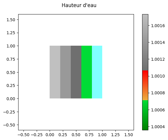
Affichage Matplotlib simple du dernier pas
[67]:
res.read_oneresult(-1)
res.set_current(views_2D.WATERDEPTH) # Calcul de la hauteur d'eau
[68]:
print('Minimum ', res[0].array.min())
print('Maximum ', res[0].array.max())

fig,ax = res[0].plot_matplotlib()
fig.suptitle('Hauteur d\'eau')
fig.colorbar(ax.images[0], ax=ax)
fig.tight_layout()
Minimum  1.0003558
Maximum  1.0017345