Analyse de plusieurs matrices sur base de polygones
Import des modules
[ ]:
try:
    from wolfhece import is_enough
    if not is_enough('2.2.31'):
        raise ImportError("Please update wolfhece to at least version 2.2.31")
except ImportError:
    raise ImportError("Please install the required version of wolfhece: pip install wolfhece>=2.2.30")

from wolfhece.analyze_poly import Arrays_analysis_zones
from wolfhece.wolf_array import WolfArray, header_wolf
from wolfhece.PyVertexvectors import vector, zone, Zones, wolfvertex as wv

import matplotlib.pyplot as plt
import numpy as np
import pandas as pd
Création de matrices de variables aléatoires
[2]:
h = header_wolf()
h.set_origin(25, 55) # Set the origin (lower-left) of the array
h.set_resolution(0.5 , 0.5) # Set the resolution of the array
h.shape = (1000, 2000) # Set the shape of the array (cells along x and y axes)
a = WolfArray(srcheader= h)
b = WolfArray(srcheader= h)
c = WolfArray(srcheader= h)
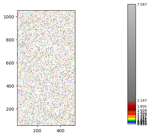
a.array[:,:] = np.random.gamma(shape = 1., scale = .5, size = 1000 * 2000).reshape((1000, 2000))
a.mask_lower(.8)
a.set_nullvalue_in_mask()
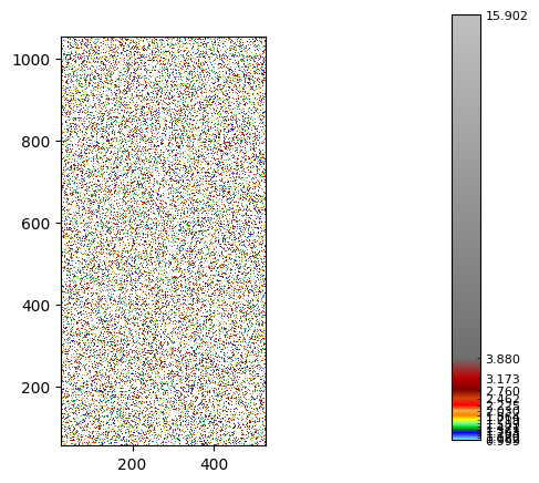
b.array[:,:] = np.random.gumbel(loc = 0., scale = 1., size = 1000 * 2000).reshape((1000, 2000))
b.mask_lower(.999)
b.set_nullvalue_in_mask()
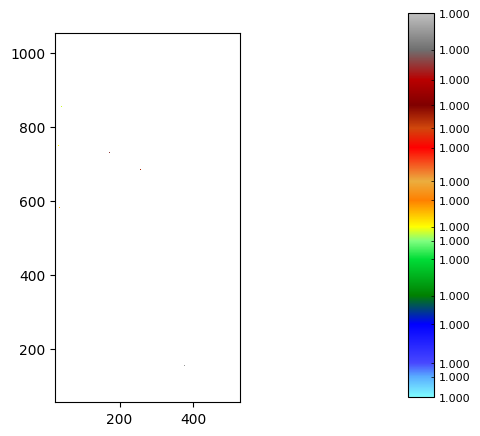
c.array[:,:] = np.random.rand(1000, 2000)
c.mask_lower(.9999)
c.set_nullvalue_in_mask()
a.plot_matplotlib(with_legend= True)
b.plot_matplotlib(with_legend= True)
c.plot_matplotlib(with_legend= True)
print("Number of values in the array:", a.nbnotnull)
print("Number of values in the array:", b.nbnotnull)
print("Number of values in the array:", c.nbnotnull)
Number of values in the array: 403990
Number of values in the array: 616406
Number of values in the array: 187
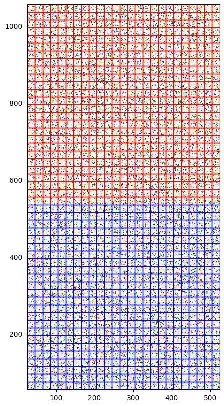
Création de polygones d’analyse
Pour l’exemple, on va définir des polygones réguliers mais répartis en 2 zones.
[ ]:
# Create polygons
zones_poly = Zones(idx = 'polygons')

zone_down = zone(name=f'Downstream_Zone')
zone_upst = zone(name=f'Upstream_Zone')

zones_poly.add_zone(zone_down, forceparent= True)
zones_poly.add_zone(zone_upst, forceparent= True)

[xmin, xmax], [ymin, ymax] = bounds = h.get_bounds()
size = 20
for x in range(int(xmin), int(xmax), size):
    for y in range(int(ymin), int(ymax), size):
        vec = vector(name=f'Vertex_{x}_{y}')
        if y > ymax // 2:  # Alternate zones based on coordinates
            vec .add_vertices_from_array(np.array([[x, y],
                                                   [x + size, y],
                                                   [x + size, y + size],
                                                   [x, y + size]]))
            vec.force_to_close()
            zone_down.add_vector(vec, forceparent= True)
        else:
            vec.add_vertices_from_array(np.array([[x, y],
                                                   [x + size, y],
                                                   [x + size, y + size],
                                                   [x, y + size]]))
            vec.force_to_close()
            zone_upst.add_vector(vec, forceparent= True)

for vec in zone_down.myvectors:
    vec.myprop.color = (255, 0, 0)  # Red for downstream zone
for vec in zone_upst.myvectors:
    vec.myprop.color = (0, 0, 255)  # Blue for upstream zone

fig, ax = plt.subplots(figsize=(10, 10))
a.plot_matplotlib(figax = (fig, ax))
zones_poly.plot_matplotlib(ax)
ax.set_aspect('equal')

print("Number of polygons in the zone down:", zone_down.nbvectors)
print("Number of polygons in the zone upst:", zone_upst.nbvectors)
Number of polygons in the zone down: 650
Number of polygons in the zone upst: 600
Création de l’objet d’analyse
Il est possible de définir un buffer autour des polygones. Le buffer est une zone supplémentaire qui permet d’inclure des valeurs adjacentes aux polygones dans l’analyse.
Si un buffer est défini, le polygone sera une copie du polygone original avec un buffer de la taille définie. Autrement, le polygone est un pointeur vers le polygone original.
[ ]:
# On passe les matrices sous la forme d'un dictionnaire dont les clés seront exploités pour les légendes
analyze = Arrays_analysis_zones(arrays= {'T2' : a, 'T25': b, 'T50' : c},
                                zones= zones_poly)
Comptage du nombre de polygones avec valeurs
Récupération sous le forme d’un dictionnaire
Récupération sous la forme d’un DataFrame pandas
[5]:
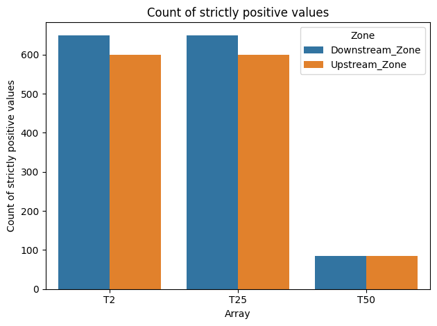
analyze.count_strictly_positive()
[5]:
{'Downstream_Zone': {'T2': 650, 'T25': 650, 'T50': 85},
 'Upstream_Zone': {'T2': 600, 'T25': 600, 'T50': 84}}
[6]:
df = analyze.count_strictly_positive_as_df()
print(df)
              Zone Array  Count
0  Downstream_Zone    T2    650
1  Downstream_Zone   T25    650
2  Downstream_Zone   T50     85
3    Upstream_Zone    T2    600
4    Upstream_Zone   T25    600
5    Upstream_Zone   T50     84
Il est possible de fusionner les différentes zones pour n’obtenir qu’un scalaire par matrice.
[7]:
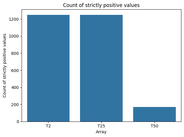
df = analyze.count_strictly_positive_as_df(merge_zones= True)
print(df.head())
  Array  Count
0    T2   1250
1   T25   1250
2   T50    169
Graphique du nombre de polygones contenant des valeurs strictement positives
Il est possible d’appeler les routines graphiques sans passer d’arguments. Toutefois, on peut :
spécifier le moteur de rendu (seaborn ou plotly)
indique si on souhaite fusionner les zones
La rouine retourne également :
pour seaborn : un tuple (fig, ax) Matplotlib
pour plotly : un objet fig plotly
Ce retour permet de retravailler le graphique le cas échéant (adaptation de la police, de la taille des axes, du grid…).
[8]:
analyze.plot_count_strictly_positive()
[8]:
(<Figure size 640x480 with 1 Axes>,
 <Axes: title={'center': 'Count of strictly positive values'}, xlabel='Array', ylabel='Count of strictly positive values'>)
Avec fusion des zones…
[9]:
analyze.plot_count_strictly_positive(merge_zones= True)
[9]:
(<Figure size 640x480 with 1 Axes>,
 <Axes: title={'center': 'Count of strictly positive values'}, xlabel='Array', ylabel='Count of strictly positive values'>)
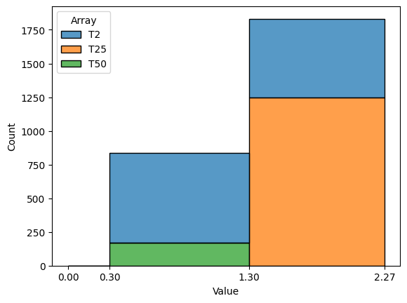
Graphique de la distribution des valeurs
Il est possible de choisir entre :
‘Mean’
‘Median’
‘Std’
‘Sum’
‘Volume’
Les intervalles par défaut sont [0., 0.3, 1.3, -1].
Terminer les ‘bins’ par -1 ajustera automatiquement la borne supérieure à la valeur maximale.
Il est possible de définir des ‘bins’ spécifiques en fournissant l’argument à la routine.
[10]:
analyze.plot_distributed_values(operator= 'Mean',
                                merge_zones= True,
                                engine= 'seaborn')
[10]:
(<Figure size 640x480 with 1 Axes>, <Axes: xlabel='Value', ylabel='Count'>)
Si on ne fusionne pas les zones, un graphique par zone sera généré.
[11]:
figs, axs = analyze.plot_distributed_values(operator= 'Mean',
                                            merge_zones= False)

print("Number of figures:", len(figs))
print("Number of axes:", len(axs))
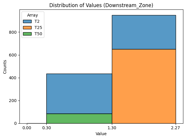
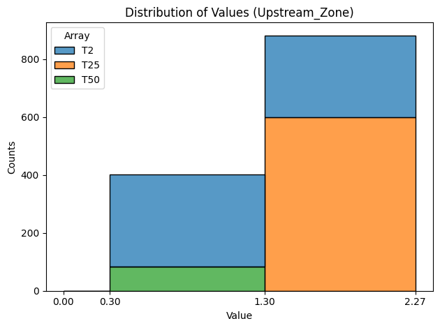
Number of figures: 2
Number of axes: 2