Analyse d’une matrice sur base de polygones et buffer

Import des modules

# import _add_path # for debugging purposes only - can be removed in production

try:
    from wolfhece import is_enough
    if not is_enough('2.2.31'):
        raise ImportError("Please update wolfhece to at least version 2.2.31")
except ImportError:
    raise ImportError("Please install the required version of wolfhece: pip install wolfhece>=2.2.30")

from wolfhece.analyze_poly import Array_analysis_polygons, Array_analysis_onepolygon
from wolfhece.wolf_array import WolfArray, header_wolf
from wolfhece.PyVertexvectors import vector, zone, Zones, wolfvertex as wv

import matplotlib.pyplot as plt
import numpy as np

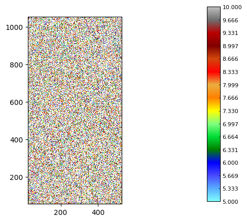
Création d’une matrice de variables aléatoires

h = header_wolf()
h.set_origin(25, 55) # Set the origin (lower-left) of the array
h.set_resolution(0.5 , 0.5) # Set the resolution of the array
h.shape = (1000, 2000) # Set the shape of the array (cells along x and y axes)

a = WolfArray(srcheader= h)

a.array[:,:] = np.random.rand(1000, 2000) * 10
a.mask_lower(5.)
a.set_nullvalue_in_mask()

a.plot_matplotlib(with_legend= True)
print("Number of values in the array:", a.nbnotnull)

Number of values in the array: 999532

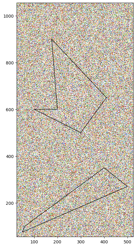
Création de polygones d’analyse

Pour l’exemple, on va définir deux polygones.

# Create polygons
zone_poly = zone(name = 'polygons')

poly1 = vector(name=f'Polygon_1', parentzone=zone_poly)
poly1.add_vertices_from_array(np.array([[60, 100],
                                        [400, 350],
                                        [500, 270],
                                        [50, 75]]))
poly1.force_to_close()  # Ensure the polygon is closed

poly2 = vector(name=f'Polygon_2', parentzone=zone_poly)
poly2.add_vertices_from_array(np.array([[410, 650],
                                        [175, 900],
                                        [200, 600],
                                        [100, 600],
                                        [300, 500]]))
poly2.force_to_close()  # Ensure the polygon is closed

zone_poly.add_vector(poly1)
zone_poly.add_vector(poly2)

fig, ax = plt.subplots(figsize=(10, 10))
a.plot_matplotlib(figax = (fig, ax))
zone_poly.plot_matplotlib(ax)
ax.set_aspect('equal')

Création de l’objet d’analyse avec buffer

Il est possible de définir un buffer autour des polygones. Le buffer est une zone supplémentaire qui permet d’inclure des valeurs adjacentes aux polygones dans l’analyse.

Si un buffer est défini, le polygone sera une copie du polygone original avec un buffer de la taille définie. Autrement, le polygone est un pointeur vers le polygone original.

analyze = Array_analysis_polygons(a, zone_poly, buffer_size= 50.)

fig, ax = plt.subplots(figsize=(10, 10))
a.plot_matplotlib(figax = (fig, ax))
analyze.polygons.plot_matplotlib(ax)
ax.set_aspect('equal')

Analyse d’un polygone spécifique

Il est possible de générer un graphique pour chaque polygone.

Au besoin, les clés des polygones peuvent être récupérées avec la propriété keys.

analyze.keys

['Polygon_1', 'Polygon_2']

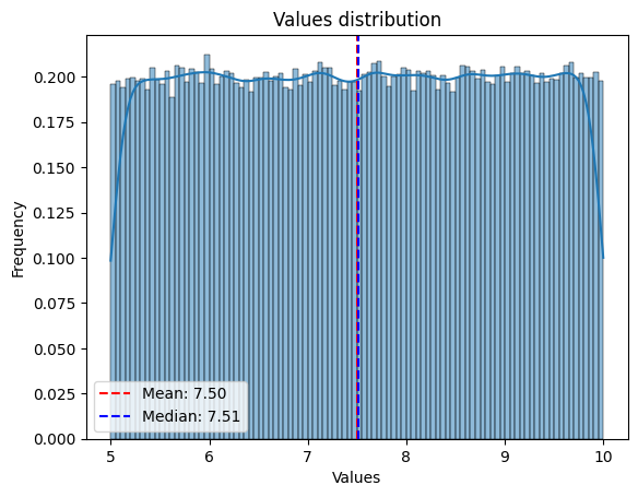
all_plots = analyze['Polygon_1'].plot_values()
all_plots = analyze['Polygon_2'].plot_values()

print('Volume Poly1 : ', analyze['Polygon_1'].values('Volume'))
print('Volume Poly2 : ', analyze['Polygon_2'].values('Volume'))

Volume Poly1 :  325365.2
Volume Poly2 :  431380.8

Récupération des coordonnées des mailles dans un polygone

et ensuite des valeurs sur base de ces coordonnées.

analyze['Polygon_1'].select_cells(mode = 'polygon')
print('Number of cells in Polygon_1:', analyze['Polygon_1'].n_selected_cells)

# get values "manually"
values = [a.get_value(x, y, convert_to_float=False) for x,y in analyze['Polygon_1'].get_selection()]
print('Values in Polygon_1:', values[:10]) # just print first 10 values

Number of cells in Polygon_1: 173679
Values in Polygon_1: [np.float32(6.318269), np.float32(7.2763643), np.float32(7.772545), np.float32(6.8120513), np.float32(7.3207436), np.float32(5.691848), np.float32(7.083117), np.float32(9.185118), np.float32(8.112824), np.float32(8.33562)]

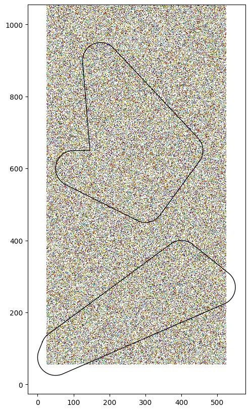
Masquer une portion de matrice sur base d’un vecteur

• Définir un vecteur central

• Utiliser des parallèles pour définir un polygone

• Masquer les valeurs de la matrice qui sont à l’intérieur du polygone

river = vector(name='River')
river.add_vertices_from_array(np.array([[100, 100],
                                         [400, 200],
                                         [400, 800],
                                         [200, 700],
                                         [300, 1000]]))

left = river.parallel_offset(25., side='left')
right = river.parallel_offset(25., side='right')
right.reverse()  # Reverse the right side to close the polygon correctly
river_poly = left + right
river_poly.force_to_close()  # Ensure the polygon is closed

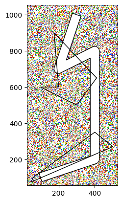
a.mask_insidepoly(river_poly)

fig, ax = a.plot_matplotlib()
river_poly.plot_matplotlib(ax)
poly1.plot_matplotlib(ax)
poly2.plot_matplotlib(ax)

analyze.update_values()
all_plots = analyze['Polygon_1'].plot_values()
all_plots = analyze['Polygon_2'].plot_values()

analyze['Polygon_1'].select_cells(mode = 'polygon')
print('Number of cells in Polygon_1:', analyze['Polygon_1'].n_selected_cells)

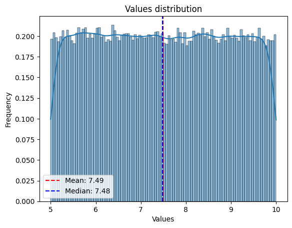
Number of cells in Polygon_1: 121939

Extraire d’autres grandeurs

Pour chaque polygone, il est calculé :

• la moyenne des valeurs (opérateur Mean)

• l’écart-type des valeurs (opérateur Std)

• la médiane des valeurs (opérateur Median)

• la somme des valeurs (opérateur Sum)

• le “volumme” des valeurs (somme des valeurs multipliée par la surface du polygone) (opérateur Volume)

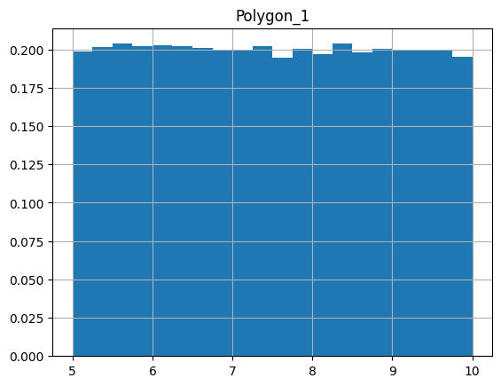
Il est toutefois possible de calculer d’autres grandeurs en exploitant la série de valeurs disponibles dans l’objet d’analyse via ‘values(‘Values’) qui retourne un DataFrame pandas.

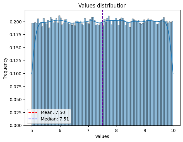
df = analyze['Polygon_1'].values('Values')
print('Type of returned object:', type(df))

print('Moyenne : ', df.mean())
print('Médiane : ', df.median())
print('Quantile 25 : ', df.quantile(0.25))
print('Quantile 75 : ', df.quantile(0.75))
print('Minimum : ', df.min())
print('Maximum : ', df.max())

df.hist(bins=20, density=True)

Type of returned object: <class 'pandas.core.frame.DataFrame'>
Moyenne :  Polygon_1    7.492949
dtype: float32
Médiane :  Polygon_1    7.48455
dtype: float32
Quantile 25 :  Polygon_1    6.239945
Name: 0.25, dtype: float32
Quantile 75 :  Polygon_1    8.743149
Name: 0.75, dtype: float32
Minimum :  Polygon_1    5.000029
dtype: float32
Maximum :  Polygon_1    9.999971
dtype: float32

array([[<Axes: title={'center': 'Polygon_1'}>]], dtype=object)