Memory Organization of NumPy Arrays

Understanding the memory layout of NumPy arrays is crucial for optimizing performance in numerical computations.

Numpy is a powerful library that provides support for large, multi-dimensional arrays and matrices, along with a collection of mathematical functions to operate on these arrays.

NumPy arrays can be stored in different memory orders, which directly impact the efficiency of operations depending on the access pattern.

This section introduces the concepts of memory organization, including C-contiguous and F-contiguous layouts, and their implications for computational performance.

Fortran or C Numpy array - Why is it important?

The Fortran or C Numpy array can be important because it allows for efficient numerical computations in Python.

The underlying implementation of Numpy is often in C or Fortran, which allows for high performance and speed when performing numerical operations.

import numpy as np
import time
import matplotlib.pyplot as plt

Multiple conventions

In NumPy, arrays can be stored in two different memory layouts:

1. C-order (row-major): Rows are stored one after the other in memory.

2. F-order (column-major): Columns are stored one after the other in memory.

a = np.array([[1,2,3],
              [4,5,6],
              [7,8,9]], order='C')

b = np.array([[1,2,3],
              [4,5,6],
              [7,8,9]], order='F')

assert a[0,0] == b[0,0]
assert a[-1,-1] == b[-1,-1]

Contiguous memory

Contiguous memory refers to a block of memory that is allocated in a single, continuous segment.

This means that all the elements of an array are stored in adjacent memory locations, allowing for efficient access and manipulation of the data.

Numpy arrays can be either contiguous or non-contiguous, depending on how they are created and manipulated. Contiguous arrays are typically faster to access and process, as they take advantage of the CPU cache and memory locality.

WolfArray numpy array are coniguous in memory.

# check if a is contiguous in memory
assert a.flags['C_CONTIGUOUS'] == True
# check if b is contiguous in memory
assert b.flags['F_CONTIGUOUS'] == True

# If necessary, force the arrays to be contiguous in memory
a = np.ascontiguousarray(a)
b = np.asfortranarray(b)

Axis, what is it?

• axis = 0 is the column, first indice - ‘i’

• axis = 1 is the row, second indice - ‘j’

# Example array
example_array = np.array([[1, 2, 3],
                          [4, 5, 6],
                          [7, 8, 9]])

print("Original Array:")
print(example_array)

# Sum along axis 0 (column-wise)
sum_axis_0 = np.sum(example_array, axis=0)
print("\nSum along axis 0 (column-wise):")
print(sum_axis_0)

# Sum along axis 1 (row-wise)
sum_axis_1 = np.sum(example_array, axis=1)
print("\nSum along axis 1 (row-wise):")
print(sum_axis_1)

Original Array:
[[1 2 3]
 [4 5 6]
 [7 8 9]]

Sum along axis 0 (column-wise):
[12 15 18]

Sum along axis 1 (row-wise):
[ 6 15 24]

Is One Axis Faster?

# Creating a 2D array
array = np.ones((500, 500))  # Large array for performance testing
for i in range(500):
    array[i, :] = i  # Fill with values
# print("Original Array:")
# print(array)

sum_colwise = np.sum(array, axis=0)  # sum all elements in each column
sum_rowwise = np.sum(array, axis=1)  # sum all elements in each row

# C-ordered array
c_ordered = np.ascontiguousarray(array)
print("\nC-ordered Array:")
# print(c_ordered)
print("Memory layout (C-order):", c_ordered.flags['C_CONTIGUOUS'])

# F-ordered array
f_ordered = np.asfortranarray(array)
print("\nF-ordered Array:")
# print(f_ordered)
print("Memory layout (F-order):", f_ordered.flags['F_CONTIGUOUS'])

# Accessing elements
print("\nAccessing elements in C-order and F-order:")
print("C-order (row-major): Accessing elements row by row is faster.")
print("F-order (column-major): Accessing elements column by column is faster.")

# Performance comparison

niter = 10_000
# Timing C-order access
start = time.time()
for _ in range(niter):
    c_sum = np.sum(c_ordered, axis=1)  # Row-wise sum
end = time.time()
print("\nTime taken for row-wise sum (C-order):", end - start)

start = time.time()
for _ in range(niter):
    c_sum = np.sum(c_ordered, axis=0)  # Column-wise sum
end = time.time()
print("Time taken for column-wise sum (C-order):", end - start)


# Timing F-order access
start = time.time()
for _ in range(niter):
    f_sum = np.sum(f_ordered, axis=1)  # Row-wise sum
end = time.time()
print("\nTime taken for row-wise sum (F-order):", end - start)

start = time.time()
for _ in range(niter):
    f_sum = np.sum(f_ordered, axis=0)  # Column-wise sum
end = time.time()
print("Time taken for column-wise sum (F-order):", end - start)

C-ordered Array:
Memory layout (C-order): True

F-ordered Array:
Memory layout (F-order): True

Accessing elements in C-order and F-order:
C-order (row-major): Accessing elements row by row is faster.
F-order (column-major): Accessing elements column by column is faster.

Time taken for row-wise sum (C-order): 1.4357905387878418
Time taken for column-wise sum (C-order): 0.8995132446289062

Time taken for row-wise sum (F-order): 1.0720064640045166
Time taken for column-wise sum (F-order): 1.4215028285980225

Observation

C-contiguous arrays in NumPy are stored in row-major order, meaning rows are stored sequentially in memory. When performing column-wise operations like np.sum(array, axis=0), the operation accesses non-contiguous memory locations, which can be slower due to cache inefficiency.

The surprising efficiency of column-wise summation (np.sum(array, axis=0)) in C-contiguous arrays, despite accessing non-contiguous memory locations, is due to NumPy’s internal optimizations. NumPy leverages highly optimized C libraries (like BLAS) that use advanced techniques such as vectorization and multi-threading to minimize the performance penalty of non-contiguous memory access. These optimizations make column-wise operations faster than expected, even though row-wise operations are inherently more cache-friendly in C-contiguous arrays.

Thus, C-order is generally more efficient for row-wise operations, while F-order is more efficient for column-wise operations. However, the best approach is to test and measure performance for your specific use case.

Optimization is not an easy task!

Memory/Matrice view

import _add_path
from wolfhece.assets.mesh import Mesh2D, header_wolf

h = header_wolf()
h.shape = (4, 3) # 4 rows, 3 columns

# Geometry - necessary for correct plotting
h.set_resolution(1., 1.)
h.set_origin(0., 0.)

# Mesh2D object from header
grid = Mesh2D(h)

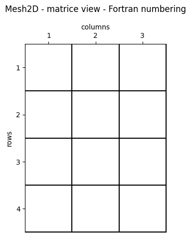
Matrice View - Fortran Numbering (1-Based)

The first element (1, 1) is the top-left one. This is the main convention in numerical analysis, image processing, and, more generally, in informatics.

fig, ax = grid.plot_cells(transpose=True)
grid.set_ticks_as_matrice(ax)
fig.suptitle("Mesh2D - matrice view - Fortran numbering")
fig.tight_layout()

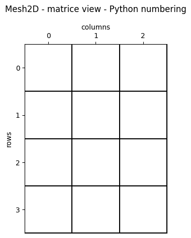
Matrice view - Python numbering (0-based)

The first element (0, 0) is the top-left one.

fig, ax = grid.plot_cells(transpose=True)
grid.set_ticks_as_matrice(ax, Fortran_type= False)
fig.suptitle("Mesh2D - matrice view - Python numbering")
fig.tight_layout()

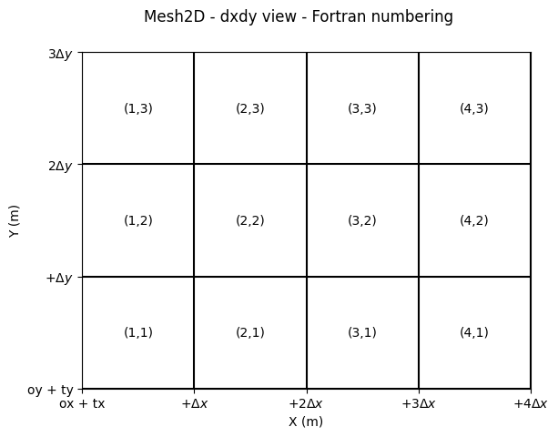
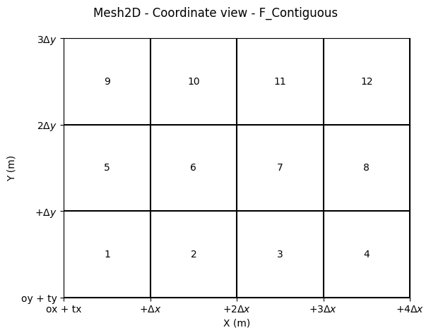
Coordinates equivalence

In a WolfArray object, we use rows as X-axis and columns as Y-axis.

The first element is the lower-left one.

The transformations between “matrice” and “coordinate” view are, in that order:

1. transpose

2. flipud

fig, ax = grid.plot_cells()
grid.set_ticks_as_dxdy(ax)
grid.plot_indices_at_centers(ax, Fortran_type=True)
fig.suptitle("Mesh2D - dxdy view - Fortran numbering")

Text(0.5, 0.98, 'Mesh2D - dxdy view - Fortran numbering')

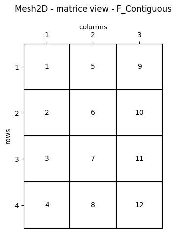
WolfArray is F_CONTIGUOUS

The NumPy array contained in a WolfArray is F_CONTIGUOUS, also known as column-major order.

This design choice stems from the fact that the WOLF code is primarily written in Fortran, which uses column-major order for storing arrays.

The WolfArray Python class is specifically designed to maintain full compatibility with its Fortran counterpart, ensuring seamless integration and efficient memory access.

It is important in memory exchange between Python and Fortran through DLL (Dynamic Link Library) and Ctypes library.

fig, ax = grid.plot_cells(transpose=True)
grid.set_ticks_as_matrice(ax, Fortran_type=True)
grid.plot_memoryposition_at_centers(ax, transpose=True, Fortran_type=True)

fig.suptitle("Mesh2D - matrice view - F_Contiguous")
fig.tight_layout()

fig, ax = grid.plot_cells(transpose=False)
grid.set_ticks_as_dxdy(ax, Fortran_type=True)
grid.plot_memoryposition_at_centers(ax, transpose=False, Fortran_type=True)

fig.suptitle("Mesh2D - Coordinate view - F_Contiguous")
fig.tight_layout()

Shape (nbx, nby) or (nby, nbx)?

When considering the “classical” or informatics convention, the X-axis corresponds to columns, and the Y-axis corresponds to rows.

The C_CONTIGUOUS memory layout is more common and is the default convention in NumPy. This layout stores rows sequentially in memory, making row-wise operations more efficient.

This convention aligns with:

• Shape: (nby, nbx) (rows, columns)

• Memory Layout: C_CONTIGUOUS (row-major order)

In contrast, the Fortran-style F_CONTIGUOUS layout stores columns sequentially in memory, which is often preferred in numerical analysis and scientific computing.

h2 = header_wolf()
h2.shape = (3, 4) # 3 rows, 4 columns

# Geometry - necessary for correct plotting
h2.set_resolution(1., 1.)
h2.set_origin(0., 0.)

Memory organization of a NumPy array in C_CONTIGUOUS order

grid2 = Mesh2D(h2)

fig, ax = grid2.plot_cells(transpose=True)
grid2.set_ticks_as_matrice(ax, Fortran_type=True)
grid2.plot_memoryposition_at_centers(ax, transpose=True, Fortran_type=True, f_contiguous=False)

(<Figure size 640x480 with 1 Axes>, <Axes: xlabel='columns', ylabel='rows'>)

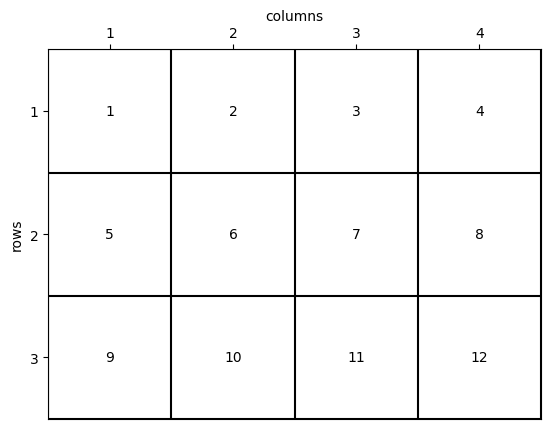
Difference Between C_CONTIGUOUS and F_CONTIGUOUS

Without delving into unnecessary technical details for this tutorial, it is important to note that the two matrix views described above result in the same memory organization.

The distinction is more about programming conventions and habits rather than performance considerations. However, understanding these conventions can help optimize code for specific use cases and improve compatibility with external libraries or systems.

Are you convinced this memory representation matches the one used in WolfArray?

For reference, in WolfArray:

• Shape: (nbx, nby)

• Memory Layout: F_CONTIGUOUS (column-major order)

This implies that one view is simply the transpose of the other. However, this transformation does not require any memory rearrangement, meaning:

• No copy is made.

• No CPU time is consumed.

Efficient and elegant!

Test on a small example

a = np.array([[1, 2, 3],
              [4, 5, 6],
              [7, 8, 9]])

# is C_contiguous?
print("C_contiguous:", a.flags['C_CONTIGUOUS'])

b = np.asfortranarray(a.T)
print("F_contiguous:", b.flags['F_CONTIGUOUS'])

# check memory location - first element of the array
print("\nMemory location of a:", a.__array_interface__['data'][0])
print("Memory location of b:", b.__array_interface__['data'][0])

print('Same memory location:', a.__array_interface__['data'][0] == b.__array_interface__['data'][0])

# Number of bytes in the array
print("\nNumber of bytes in a:", a.nbytes)
print("Number of bytes in b:", b.nbytes)

# Ravel the arrays - Return a contiguous flattened array without copying data
# (if possible)
# NOT the same as flatten() - which returns a copy of the array
a_ravel = a.ravel()
b_ravel = b.ravel()

print("\nIs first element the same ?", a_ravel[0] == b_ravel[0])
print("Is last element the same ?", a_ravel[-1] == b_ravel[-1])

C_contiguous: True
F_contiguous: True

Memory location of a: 2402888579840
Memory location of b: 2402888579840
Same memory location: True

Number of bytes in a: 72
Number of bytes in b: 72

Is first element the same ? True
Is last element the same ? True