Convolution

A convolution operation is a mathematical operation used in various fields such as signal processing, image processing, and machine learning. It involves combining two functions to produce a third function that expresses how the shape of one is modified by the other.

In this tutorial, we want to explore and compare different implementations of 2D convolution.

We will implement 2D convolution in Python using various libraries. Specifically, we will look at three different methods: scipy_fft, jax_fft, and scipy_convolve2d.

The total time taken by each method will be measured and compared.

Import necessary libraries

import numpy as np
import matplotlib.pyplot as plt
from wolfhece.wolf_array import header_wolf, WolfArray

from datetime import datetime as dt, timedelta

Creation of a matrix and a filter

def set_a_f(n, n_filter):
    h = header_wolf()
    h.shape = (n, n)
    h.set_resolution(0.1, 0.1)

    h_filter = header_wolf()
    h_filter.shape = (n_filter, n_filter)
    h_filter.set_resolution(0.1, 0.1)

    a = WolfArray(srcheader=h)
    f = WolfArray(srcheader=h_filter)

    return a, f

Setting up data for different cases

to_test = [(100, 10),
           (200, 20),
           (500, 50),
           (1000, 100),
           (2000, 200),
           (5000, 500),
        #    (10000, 1000),
           ]

all = [set_a_f(n, n_filter) for n, n_filter in to_test]

Calculation of the convolution with Numpy

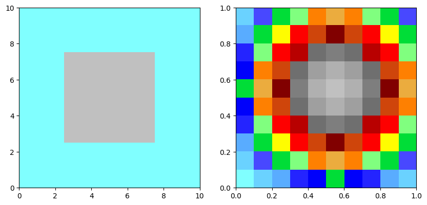
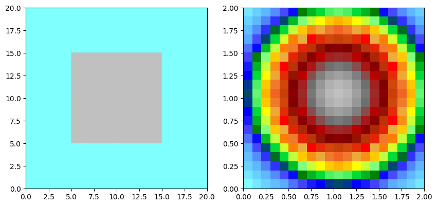
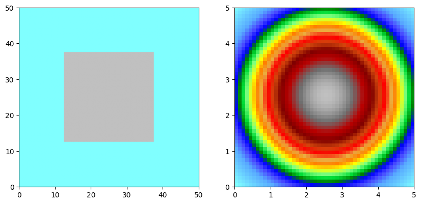
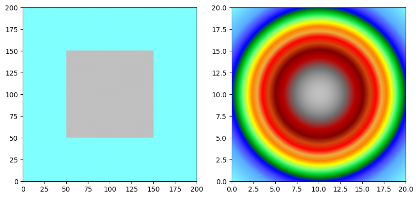
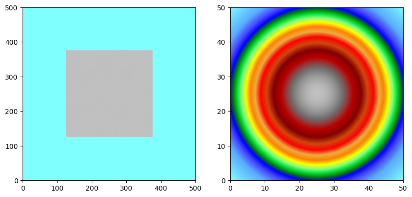
for a, f in all:
    fig, axes= plt.subplots(1, 2, figsize=(10, 5))
    n = a.shape[0]
    a.array[n//2-n//4:n//2+n//4,n//2-n//4:n//2+n//4] = 2.0
    a.plot_matplotlib((fig, axes[0]))
    # make a circular filter with exponential falloff
    n_filter = f.shape[0]
    f.array[:,:] = np.asarray([np.exp(-((i-n_filter/2)**2+(j-n_filter/2)**2)/n_filter**2) for i in range(n_filter) for j in range(n_filter)]).reshape((n_filter,n_filter))
    f.plot_matplotlib((fig, axes[1]))
    plt.show()

Calculation of convolution using Fourier transform

For larger matrices, convolution can be computed more efficiently using the Fast Fourier Transform (FFT).

We test two implementations: one using scipy.fft and another using jax.numpy.fft.

• scipy_fft

• jax_fft

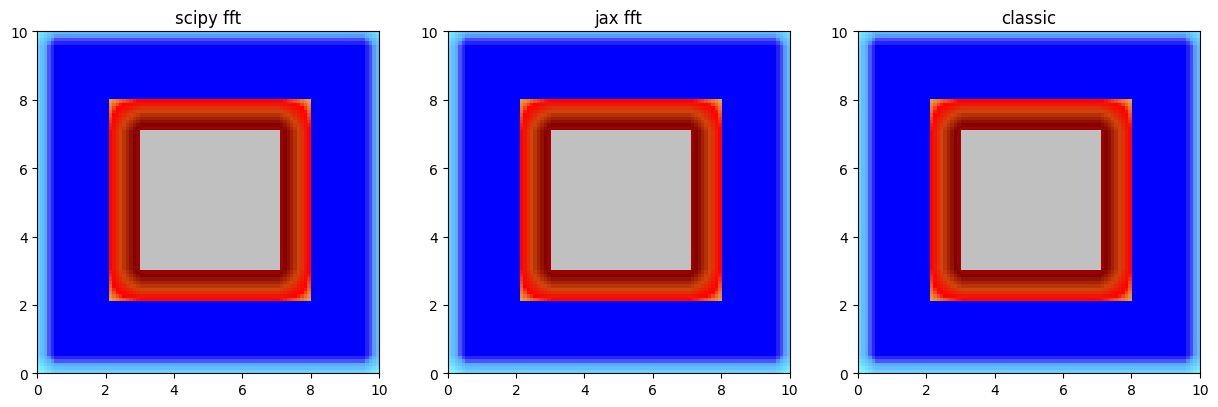
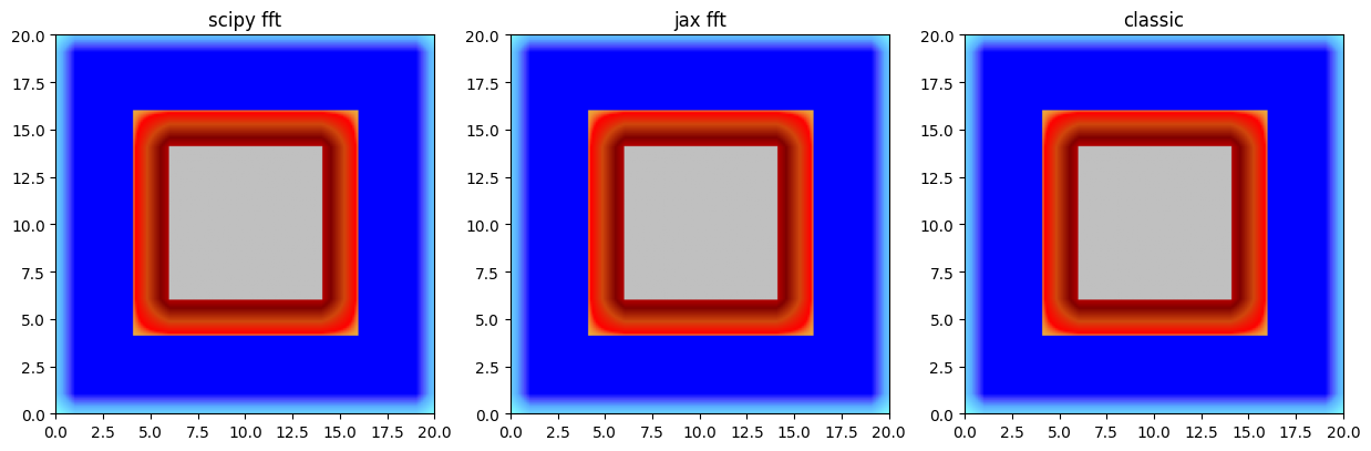
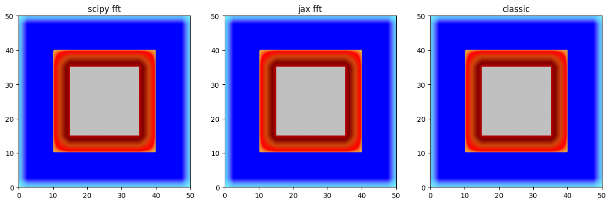
for a, f in all:
      fig, axes = plt.subplots(1, 3, figsize=(15, 5))

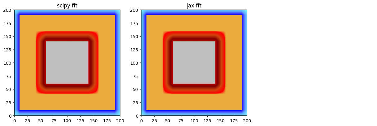
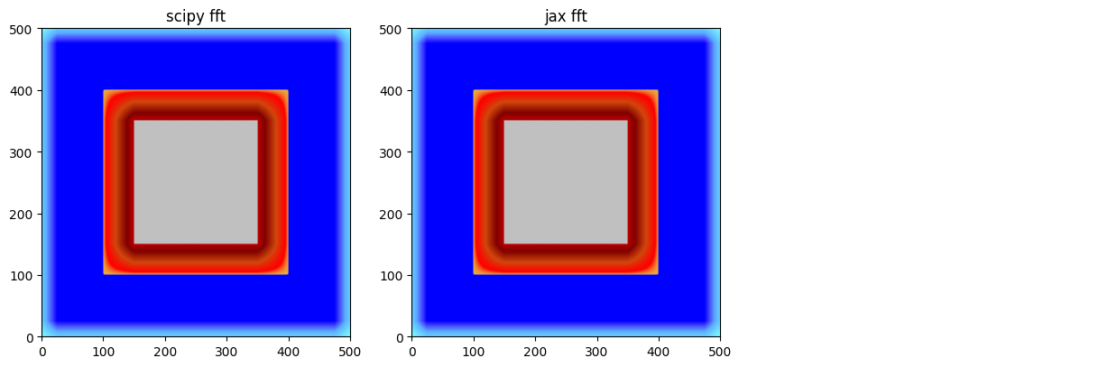
      # scipy fft
      start = dt.now()
      scipy_fft = a.convolve(f, method='scipyfft', inplace=False)
      scipy_runtime = dt.now() - start
      scipy_fft.plot_matplotlib((fig, axes[0]))
      axes[0].set_title('scipy fft')

      # jax fft
      start = dt.now()
      jax_fft = a.convolve(f, method='jaxfft', inplace=False)
      jax_runtime = dt.now() - start
      jax_fft.plot_matplotlib((fig, axes[1]))
      axes[1].set_title('jax fft')

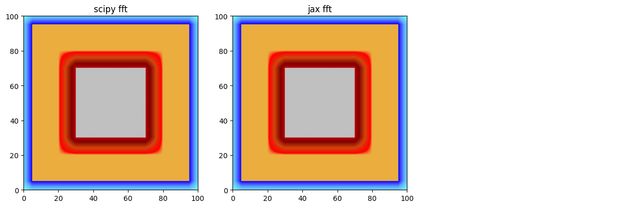
      if a.shape[0] <= 500:
            #classic == scipy.convolve2d
            start = dt.now()
            classic = a.convolve(f, method='classic', inplace=False)
            classic_runtime = dt.now() - start
            classic.plot_matplotlib((fig, axes[2]))
            axes[2].set_title('classic')
      else:
            classic_runtime = timedelta(0)
            axes[2].axis('off')

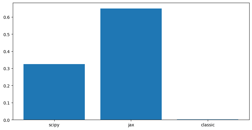
      plt.figure(figsize=(10, 5))
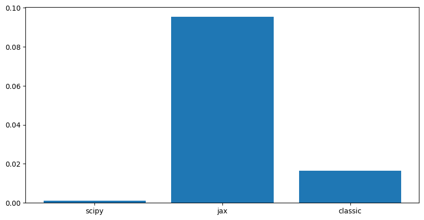
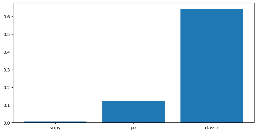
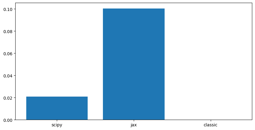
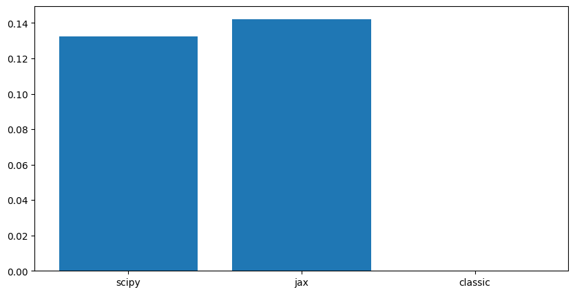
      plt.bar([0,1,2], [scipy_runtime.total_seconds(),
                        jax_runtime.total_seconds(),
                        classic_runtime.total_seconds()],
                  tick_label=['scipy', 'jax', 'classic'])
      plt.show()

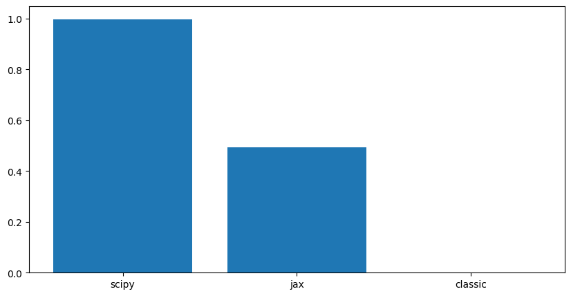
Conclusions

Computattion time evolves with the size of the matrix and the filter.

For very large matrices, the FFT-based methods are significantly faster than the direct convolution method.

Jax only outperforms Scipy for very large matrices, likely due to its optimization for GPU acceleration. But for smaller matrices, the overhead of using Jax may not be justified.