WolfArray, what is it?
Note — This tutorial uses the
WolfArrayclass, which includes GUI/OpenGL support. If you only need data manipulation (scripts, CI, HPC), you can useWolfArrayModelinstead — same API, no GUI dependency. See the Model/GUI architecture tutorial for details.
Basics
A WolfArray is a data structure that allows you to store and manipulate arrays of data more efficiently. It is designed to be easy to use and flexible, enabling you to work with different types of data without worrying about the underlying implementation details.
Internally, a WolfArray contains a masked numpy array (see numpy.ma) in the .array attribute. This allows you to store data in a way that is both efficient and easy to work with. The masked array enables you to handle missing or invalid data easily while still providing the performance benefits of a regular numpy array.
Georeferencing capabilities are provided by these attributes (stored in the header_wolf class, from which this class inherits):
origx,origy: The local coordinates of the lower-left corner of the array.dx,dy: The pixel size in the x and y directions, respectively.nbx,nby: The number of pixels in the x and y directions, respectively.translx,transly: The translation in the x and y directions, respectively—equal to(0., 0.)by default but can be set to any value.
(origx, origy) and (translx, transly) are summed to give the global coordinates of the lower-left corner of the array.
Maybe you known the Rasterio package? In a certain way, the WolfArray is similar to a rasterio dataset, but it is designed to be more flexible and fully compatible with WOLF.
Numpy Considerations
The masked numpy array is:
Fortran contiguous (F-order), so the first index evolves the fastest.
nbxis the number of rows (first index).nbyis the number of columns (second index).The first element of the array
(0, 0)is at the(origx + dx / 2., origy + dy / 2.)coordinates, eventually translated by(translx, transly).The element
(i, j)is at the(origx + dx / 2. + i * dx, origy + dy / 2. + j * dy)coordinates, eventually translated by(translx, transly).
So, the X-axis corresponds to the first index, and the Y-axis corresponds to the second index. This is important to remember when working with the WolfArray, as it can affect how you access and manipulate the data.
This is not the classical way of storing 2D data in Python, where the first index is the row and the second index is the column. However, this design choice was made for Fortran compatibility, and it is important to keep this in mind when working with the WolfArray. Retrocompatibility is important!
You can use the transpose method to convert the array to the classical way of storing 2D data in Python, but this is not recommended unless absolutely necessary.
Based on this design, the indices of the array [i, j] can be viewed as the [x, y] position. i varies along the X-axis, and j varies along the Y-axis.
Viewer Compatibility
The WolfArray is designed to be compatible with the WolfMapviewer.
The class inherits from the Element_to_Draw class, which unifies the minimal interface of objects that can be drawn in the viewer.
Plotting
A WolfArray can be plotted in the viewer using the plot method (OpenGL accelerated).
In a script, you can use the plot_matplotlib method to plot the data using Matplotlib.
Python/Fortran
As Wolf uses both Python and Fortran, the WolfArray is designed to be compatible with both languages.
You will find in some routines an aswolf parameter. If True, the routine will use/return a Fortran 1-based numeration, and if False, it will use a Python 0-based numeration.
This is important to remember when working with the ``WolfArray``, as it can affect how you access and manipulate the data.
Data types
A WolfArray can store different types of data, including:
int: Integer (int8, uint8, int16, int32)float: Floating-point (float32 - by default, float64)bool: Boolean/Logical
Informations can be obtained using the dtype attribute or wolftype, which returns the data type of the array.
dtype is a numpy dtype object, while wolftype is an integer representation of the data type.
How to create a WolfArray?
[1]:
# import the module
from wolfhece.wolf_array import WolfArray, header_wolf

# create a header object
h = header_wolf()
# Define some parameters
h.set_origin(10., 50.) # (origx, origy)
h.set_resolution(0.5, 0.5) # (dx, dy)
h.shape = (100, 100) # (nbx, nby)

wa = WolfArray(srcheader=h)
[2]:
# print infos
print(wa)
Shape  : 100 x 100
Resolution  : 0.5 x 0.5
Spatial extent :
   - Origin : (10.0 ; 50.0)
   - End : (60.0 ; 100.0)
   - Width x Height : 50.0 x 50.0
   - Translation : (0.0 ; 0.0)
Null value : 0.0
Type order - C or F ?
[3]:
print('Is internal array F_CONTIGUOUS? ', wa.array.flags['F_CONTIGUOUS'])
print('Is internal array C_CONTIGUOUS? ', wa.array.flags['C_CONTIGUOUS'])
Is internal array F_CONTIGUOUS?  True
Is internal array C_CONTIGUOUS?  False
NoData/NullValue, bounds, plot…
[4]:
# By default, the Numpay array is initialized with ones, not zeros.
#
# A the .array attribute is a numpy array, so you can use all the numpy functions on it.
print(wa.array.max())
print(wa.array.min())
1.0
1.0
[5]:
# find bounds
bounds = wa.get_bounds()
print("Bounds: [xmin, xmax], [ymin, ymax]", bounds)

(xmin, xmax), (ymin, ymax) = bounds
Bounds: [xmin, xmax], [ymin, ymax] ([10.0, 60.0], [50.0, 100.0])
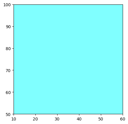
[7]:
wa.plot_matplotlib() # The plot routine uses the header informations to set the axes limits and ticks
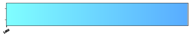
# colormap/palette is available in the .mypal attribute
# print the colormap
import matplotlib.pyplot as plt
fig, ax = plt.subplots()
wa.mypal.plot(fig, ax)
fig.set_size_inches(8,1)
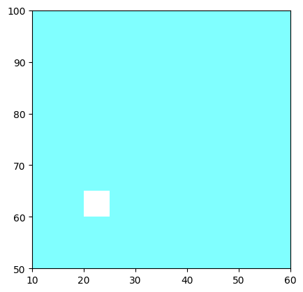
[6]:
# You can mask cells
wa.array[20:30, 20:30] = 0.
wa.mask_data(0.)
wa.plot_matplotlib()
[6]:
(<Figure size 640x480 with 1 Axes>, <Axes: >)
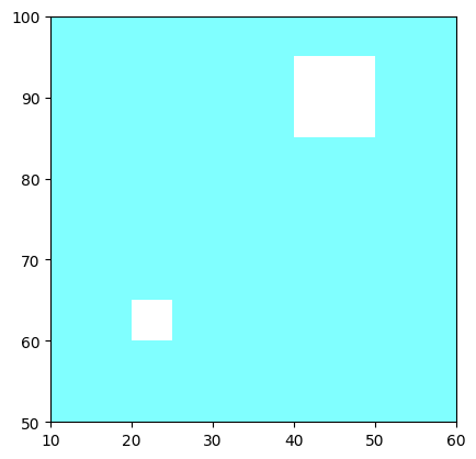
[8]:
wa.array.mask[60:80, 70:90] = True
wa.set_nullvalue_in_mask()
wa.plot_matplotlib()
[8]:
(<Figure size 640x480 with 1 Axes>, <Axes: >)
[9]:
# The Class has a NoData/NullValue attribute
# .nodata and .nullvalue are the same information (aliases)

print(wa.nullvalue)
print(wa.nodata)
0.0
0.0
[10]:
# Fill the array with linear values
import numpy as np
wa.array.data[:,:] = np.linspace(0, 1, wa.array.size).reshape(wa.array.shape) # We use the .data attribute to access the array data -- the mask is intact
wa.set_nullvalue_in_mask() # We set the nullvalue in the mask again, because we changed the data
fig, ax = wa.plot_matplotlib() # we can get the figure and axes objects from the plot function
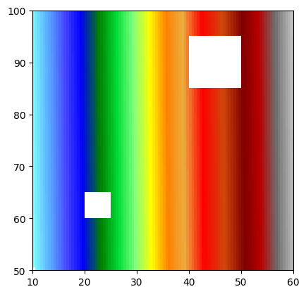
WolfArray has numerous routines to manipulate the data.
[11]:
new_wa = WolfArray(mold=wa) # We can create a new WolfArray object from an existing one, using the mold parameter
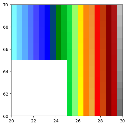
[12]:
crop_wa = WolfArray(mold=wa, crop=[[20,30],[60,70]]) # We can crop the array using the mold parameter and the crop parameter
crop_wa.plot_matplotlib() # We can plot the cropped array
[12]:
(<Figure size 640x480 with 1 Axes>, <Axes: >)
[13]:
# We can rebin (aggregation/disaggregation) the array using the rebin method.

# if
new_wa.rebin(factor = 2) # We can rebin the array using the rebin method, with a factor of 2. An operator can be set in the rebin method, default is 'mean'.
new_wa.plot_matplotlib()
print(new_wa)
Shape  : 50 x 50
Resolution  : 1.0 x 1.0
Spatial extent :
   - Origin : (10.0 ; 50.0)
   - End : (60.0 ; 100.0)
   - Width x Height : 50.0 x 50.0
   - Translation : (0.0 ; 0.0)
Null value : 0.0

[14]:
new_wa2 = WolfArray(mold=wa)
new_wa2.rebin(factor = .25)
new_wa2.plot_matplotlib()
print(new_wa2)
Shape  : 400 x 400
Resolution  : 0.125 x 0.125
Spatial extent :
   - Origin : (10.0 ; 50.0)
   - End : (60.0 ; 100.0)
   - Width x Height : 50.0 x 50.0
   - Translation : (0.0 ; 0.0)
Null value : 0.0

A WolfArray can read and write data to and from various file formats, including .bin (Wolf Binary), .tif/.tiff, .vrt, .npy, and .npz.
Some formats include georeferencing information, while others do not. The WolfArray automatically detects the format and processes the data accordingly.
Internally, GDAL can be used to handle reading and writing data to and from files.
Saving and Loading
A WolfArray can be saved to disk using write_all(). The format is determined by the file extension:
.bin— Wolf binary (default).tif/.tiff— GeoTIFF (optionally with EPSG).npy— NumPy binary
To reload, simply pass the file path to the constructor: WolfArray(fname=path).
[15]:
import tempfile, os

# Save the array to a temporary Wolf binary file
tmpdir = tempfile.mkdtemp()
fpath = os.path.join(tmpdir, 'test_array.bin')

wa.write_all(fpath)
print(f"Saved to {fpath}")
print("Files created:", [f for f in os.listdir(tmpdir) if 'test_array' in f])
Saved to C:\Users\pierre\AppData\Local\Temp\tmp2miyqsam\test_array.bin
Files created: ['test_array.bin', 'test_array.bin.txt']
[16]:
# Reload from file
wa_loaded = WolfArray(fname=fpath)
print(wa_loaded)
print("Arrays equal:", np.allclose(wa.array.data, wa_loaded.array.data))
Shape  : 100 x 100
Resolution  : 0.5 x 0.5
Spatial extent :
   - Origin : (10.0 ; 50.0)
   - End : (60.0 ; 100.0)
   - Width x Height : 50.0 x 50.0
   - Translation : (0.0 ; 0.0)
Null value : 0.0


Arrays equal: True
Accessing Values by Coordinates
Use get_value(x, y) to query the array at real-world coordinates (the header handles the mapping from world coordinates to array indices).
[17]:
import numpy as np

# get_value returns the value at the given real-world coordinates
# Pick a point well inside the array and away from masked regions
val = wa.get_value(20., 70.)
print(f"Value at (20., 70.): {val}")

# Compare with direct array indexing
# (20. - 10.) / 0.5 = 20 → i=20, (70. - 50.) / 0.5 = 40 → j=40
print(f"Direct array[20, 40]: {wa.array[20, 40]}")

# Querying outside the array returns -99999 by default
val_outside = wa.get_value(0., 0.)
print(f"Value outside bounds: {val_outside}")

# Clean up temp files
import shutil
shutil.rmtree(tmpdir, ignore_errors=True)
Value at (20., 70.): 0.2040203958749771
Direct array[20, 40]: 0.2040203958749771
Value outside bounds: -99999.0