Ritter dam break solution
The Ritter dam-break solution, developed in 1892 by German engineer A. Ritter, is one of the earliest and most influential analytical models used to describe the behavior of water flow following the sudden failure of a dam. This model was inspired by catastrophic dam failures in the 19th century, particularly the South Fork Dam disaster in Johnstown, Pennsylvania, in 1889, w hich claimed over 2,000 lives.
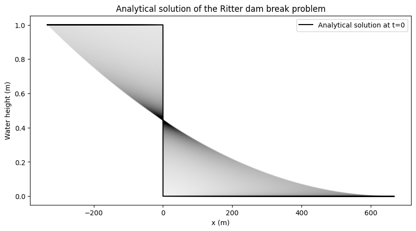
Ritter’s solution assumes an idealized scenario: a frictionless, horizontal channel with an instantaneous dam removal. Under these conditions, the water initially held behind the dam surges forward, creating a rapidly moving flood wave. The model provides exact mathematical expressions for the velocity and depth of the water as it propagates downstream.
Despite its simplifications, the Ritter solution remains a cornerstone in the study of dam-break hydraulics. It serves as a benchmark for validating more complex numerical models and helps engineers understand the fundamental dynamics of flood wave propagation
Wave celerity [m/s] : \(c_0 = \sqrt{g h_0}\)
Analytical solution : \(h(x,t) = \frac{1}{9g} \left(-\frac{x}{t}+2c_0\right)^2\)
References :
Import modules
[1]:
from pathlib import Path
import numpy as np
from wolfgpu.simple_simulation import  SimpleSimulation, SimulationDuration
from wolfgpu.SimulationRunner import SimulationRunner, load_simple_sim_to_gpu, PerformancePolicy
from wolfgpu.results_store import ResultsStore

import matplotlib.pyplot as plt

from wolfhece.wolf_array import WolfArray
Problem definition
[12]:
g = 9.81  # Gravitational acceleration
dx, dy = 0.1, 0.1 # Spatial step size
nx, ny = 10002, 5 # Number of grid points in x and y direction

idx_dam = nx // 3 # Cell index of the first cell after the dam
x_dam = idx_dam * dx + dx / 2.  # Position of the dam in x

print(f"Grid size: {nx} x {ny}, dx = {dx}, dy = {dy}")
print(f"Position of the dam break: {idx_dam} (at x = {x_dam})")

h0 = 1.0 # Initial water depth
c0 = np.sqrt(g * h0)  # Initial wave speed

t_out = 1.0  # Output time interval [s]

# abscissa for plotting
# x at idx_dam is dx / 2.0 [m]
x = np.zeros(nx)
x[idx_dam+1:] = np.arange(0, nx - idx_dam - 1) * dx + dx / 2.0  # downstream
x[:idx_dam+1] = -((np.arange(idx_dam+1) * dx)[::-1] + dx / 2.0)  # reverse order for upstream
Grid size: 10002 x 5, dx = 0.1, dy = 0.1
Position of the dam break: 3334 (at x = 333.45000000000005)
Analytical solution
[13]:
def analytical_solution(x, t):
    # between -c0*t and 2*c0*t
    if t == 0:
        h = h0 * np.ones_like(x)
        h[idx_dam+1:] = 0.0
        return h
    else:
        h = h0 * np.ones_like(x)
        h[idx_dam+1:] = 0.0
        i1 = int(-c0*t/dx)
        i2 = int(2*c0*t/dx)
        h[idx_dam+i1:idx_dam+i2] = 1/(9*g) * np.power(-x[idx_dam+i1:idx_dam+i2]/t + 2*c0, 2.0)
    return h

t_max = x[-1] / (2.*c0)  # Maximum time for the wave to reach the end
times= np.arange(0.0, t_max, t_out)
analytic = [analytical_solution(x, t) for t in times]
[14]:
fig, ax = plt.subplots(figsize=(10, 5))
for sol in analytic:
    ax.plot(x, sol, color='black', alpha=0.1)
ax.plot(x, analytic[0], color='black', label='Analytical solution at t=0')
ax.set_xlabel('x (m)')
ax.set_ylabel('Water height (m)')
ax.set_title('Analytical solution of the Ritter dam break problem')
ax.legend()
plt.show()
GPU model
[ ]:
# Create the simulation
sim = SimpleSimulation(nx = nx, ny = ny)

# Create a nap
nap = np.zeros((nx, ny), dtype=np.uint8)
nap[1:-1, 1:-1] = 1  # Set all cells to active except the border cells

# Create a bathymetry
bath = np.ones((nx, ny), dtype=np.float32) * 99999. # 99999. is a placeholder for inactive cells
bath[nap == 1] = 0.0 # Set bathymetry to 0.0 for active cells

# Create initial water depth and flow fields
h = np.zeros((nx, ny), dtype=np.float32)
h[nap == 1] = h0  # Set initial water height
h[idx_dam:,1:-1] = 0.0  # Set water height downstream

qx = np.zeros((nx, ny), dtype=np.float32)
qy = np.zeros((nx, ny), dtype=np.float32)

sim.nap = nap
sim.bathymetry = bath
sim.h = h
sim.qx = qx
sim.qy = qy
sim.manning = np.ones((nx, ny), dtype=np.float32) * 0.0  # Set Manning's n

sim.param_dx = dx
sim.param_dy = dy
sim.param_courant = 0.65 # Courant-Friedrichs-Lewy (CFL) condition - above, some oscillations may occur at the font wave
sim.param_froude_max = 20000. # Maximum Froude number
sim.param_duration = SimulationDuration.from_seconds(t_max) # Simulation duration
sim.param_report_period = SimulationDuration.from_seconds(t_out) # Output period
Check errors
[38]:
sim.check_errors()
Save model on disk
[45]:
simdir = Path('.') / "output"
simdir.mkdir(exist_ok=True)
sim.save(simdir)
Compute
[46]:
rs: ResultsStore = SimulationRunner.quick_run(sim, simdir, perf_policy= PerformancePolicy.SPEED)
[108 records] t=1 m. 47 s. Δt=0.0108s 0 dryups iter.: |██████|, 577.14 it./sec.
Extract results
[47]:
steps = list(range(2, rs.nb_results, 1)) # ignore first step which is the initial state
times = rs.get_named_series('t')[2:]

hq = [rs.get_named_result(['h', 'qx'], step) for step in steps]
h = [hq_i[0].T[:,3] for hq_i in hq] # Transpose to get the correct shape (nx, ny)
q = [hq_i[1].T[:,3] for hq_i in hq]
GPU results vs Analytics
Numerical assumptions:
Spatial finite volume scheme with constant reconstruction
Uniform spatial step size
Runge-Kutta 2steps - 2nd order
No limiter
Automatic timestep
[48]:
%matplotlib widget
# Find the front wave for each time step
front_wave = []
for h_i in h:
    front_wave.append((x[np.min(np.where((h_i<h0) & (h_i>0.)))], x[np.max(np.where(h_i>0.))]))  # Find the first index where h > 0

# Find the front wave in the analytical solution
front_wave_analytical = []
for sol in analytic[1:len(front_wave)+1]:
    front_wave_analytical.append((x[np.min(np.where(sol<h0))] ,x[np.max(np.where(sol>0.))]))  # Find the first index where h > 0

print(len(front_wave), len(front_wave_analytical))

# Plot the results
fig, ax = plt.subplots(figsize=(10, 5))
ax.scatter(front_wave_analytical[:], front_wave[:], label='Simulation front wave', color='blue', s=10)

# Add exact results
x_front_downstream = []
x_front_upstream = []
for t in times[:-1]:
    x_front_downstream.append(2. * c0 * t)
    x_front_upstream.append(-c0 * t)
ax.scatter([x_front_upstream, x_front_downstream],
           [x_front_upstream, x_front_downstream],
           label='Exact solution front wave', color='red', s= 2)

ax.set_aspect('equal')
ax.set_xlabel('Analytical front wave position (m)')
ax.set_ylabel('Simulation front wave position (m)')
ax.set_title('Front wave position of the Ritter dam break problem')
ax.legend()
plt.show()
106 106
[49]:
%matplotlib widget
fig, ax = plt.subplots(3, 1, figsize=(10, 15))
for i, h_i in enumerate(h):
    ax[0].plot(x[1:-1], h_i[1:-1], color='blue', alpha=0.1, label=f'Simulation at t={times[i]:.2f}s')
    ax[0].plot(x[1:-1], analytic[i+1][1:-1], color='black', alpha=0.1)
ax[0].plot(x[1:-1], analytic[0][1:-1], color='black', label='Simulation at t=0s')

for i, h_i in enumerate(h):
    ax[1].plot(x[1:-1], h_i[1:-1], color='blue', alpha=0.1, label=f'Simulation at t={times[i]:.2f}s')
    ax[1].plot(x[1:-1], analytic[i+1][1:-1], color='black', alpha=0.1)
ax[1].plot(x[1:-1], analytic[0][1:-1], color='black', label='Simulation at t=0s')
ax[1].set_ylim(0,0.2)
ax[1].set_xlim(0,200.)

for i, h_i in enumerate(h):
    ax[2].plot(x[1:-1], h_i[1:-1], color='blue', alpha=0.1, label=f'Simulation at t={times[i]:.2f}s')
    ax[2].plot(x[1:-1], analytic[i+1][1:-1], color='black', alpha=0.1)
ax[2].plot(x[1:-1], analytic[0][1:-1], color='black', label='Simulation at t=0s')
ax[2].set_ylim(4/9 *h0 - .1, 4/9 *h0 + 0.1)
ax[2].set_xlim(-20.,20.)

ax[2].set_xlabel('x (m)')
ax[0].set_ylabel('Water depth (m)')
ax[1].set_ylabel('Water depth (m)')
ax[2].set_ylabel('Water depth (m)')


fig.tight_layout()
[51]:
%matplotlib widget
fig, ax = plt.subplots(figsize=(5, 5))
# Scatter plot of numerical results vs analytical solution
# Plot 1 step over 5 for better visibility
for i in range(0, len(h), 5):
    ax.scatter(analytic[i+1][1:-1],
               h[i][1:-1],
               color='blue', alpha=0.5,
               marker='o', s=1)
ax.plot([0, h0], [0, h0], color='black', label='y=x line')
ax.set_xlabel('Analytical water depth (m)')
ax.set_ylabel('Simulation water depth (m)')
ax.set_title('Numerical vs Analytical water depth')
ax.legend()
plt.show()