Profile, what is it?
Basics
The profile class overrides the vector class to add some specific methods and properties.
The main goal is to be able to compute cross sections along a line (the profile) and to be able to plot them easily.
But If normaly a profile is a 2D object (X,Z) or (Y,Z), in wolfhece it is a 3D object (X,Y,Z) with some specific methods to compute cross sections.
The vertices are not necessarly aligned along a unique trace. This is useful during triangulation process where the profiles captured on the fields are not necessarly straight.
Import
[1]:
import numpy as np
from pathlib import Path
import matplotlib.pyplot as plt

from wolfhece import is_enough
if not is_enough('2.2.43'):
    raise ImportError("This code requires wolfhece version 2.2.43 or higher. -- try pip install wolfhece --upgrade")

from wolfhece.wolf_array import WolfArray, header_wolf as hw, WOLF_ARRAY_FULL_SINGLE, WOLF_ARRAY_FULL_INTEGER
from wolfhece.pydownloader import toys_dataset

from wolfhece.PyCrosssections import profile, crosssections, example_largesect, example_smallsect, example_diffsect1
from wolfhece.PyVertexvectors import Zones
How to create a profile?
A profile can be created from:
a multiline string with (X, Z) coordinates separated by spaces and each vertex on a new line,
a list of tuples (X, Z),
a list of lists (X, Z),
a NumPy array of shape (N, 2),
a list of vertices,
a WOLF vector object.
The X coordinates must not start from 0.
Except for the list of vertices and the vector, internally, (X, Z) coordinates are stored as (X, Y, Z) coordinates where Y = 0.
During plotting, (S, Z) coordinates are used, where S is the curvilinear coordinate starting from 0 at the left vertex.
Exemple 1 : a large section
Data
[2]:
print(example_largesect)
-138 100
-114 90
-70 80
-45 70
-32 62
0 61.5
32 62
60 70
80 80
98 84
120 87
Initialization
[3]:
prof_large = profile(name = 'Large profile',      # name of the profile
               data_sect=example_largesect) # data of the cross-section (list of tuples, numpy array, string filename or vector of vertices)
Plotting the cross-section
It is possible to plot the cross-section with the method plot_cs and to specify a water level with the argument fwl (for fill water level).
If fig and ax are not specified, a new figure and axis are created.
[4]:
fig, ax = plt.subplots(figsize=(10,6))
prof_large.plot_cs(fwl=90.,
             show=True,
             forceaspect=True,
             fig = fig,
             ax = ax,
             plotlaz= False,    # --> see below for more details
             clear=True,
             linked_arrays={})  # --> see below for more details
D:\ProgrammationGitLab\HECEPython\docs\source\tutorials\../../..\wolfhece\PyCrosssections.py:2281: UserWarning: FigureCanvasAgg is non-interactive, and thus cannot be shown
  fig.show()
[4]:
(-99999.0, -99999.0, -99999.0, -99999.0, -99999.0, -99999.0)

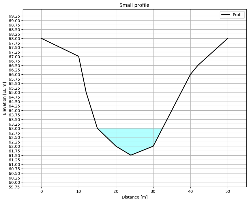
Exemple 2 : a small section
[5]:
prof_small = profile(name = 'Small profile',      # name of the profile
                     data_sect=example_smallsect) # data of the cross-section
fig, ax = plt.subplots(figsize=(10,8))
prof_small.plot_cs(fwl=63., show=True, fig = fig, ax = ax, forceaspect= False)
[5]:
(-99999.0, -99999.0, -99999.0, -99999.0, -99999.0, -99999.0)
Example 3 : a rectangular one
[6]:
prof_rect = profile(name = 'Rectangular profile',      # name of the profile
                     data_sect=[(0.,10.), (0.,0.),(10.,0.),(10.,10.)]) # data of the cross-section
fig, ax = plt.subplots(figsize=(10,5))
prof_rect.plot_cs(fwl=5., show=True, fig = fig, ax = ax, forceaspect= False)
[6]:
(-99999.0, -99999.0, -99999.0, -99999.0, -99999.0, -99999.0)

How to access the geometry ?
As a profileobject is a vector object, you can access the vertices with the property myvertices or the coordinates with the property xy or xyz.
Coordinates along the profile can be accessed with the property s (curvilinear abscissa) and z (elevation).
XYZ coordinates
The provided coordinates of the profile are stored as (X, Y, Z) coordinates where Y = 0.
[7]:
print(prof_small.xyz)
print(prof_large.xyz)
[[ 0.   0.  68. ]
 [10.   0.  67. ]
 [12.   0.  65. ]
 [15.   0.  63. ]
 [20.   0.  62. ]
 [24.   0.  61.5]
 [30.   0.  62. ]
 [35.   0.  64. ]
 [40.   0.  66. ]
 [42.   0.  66.5]
 [50.   0.  68. ]]
[[-138.     0.   100. ]
 [-114.     0.    90. ]
 [ -70.     0.    80. ]
 [ -45.     0.    70. ]
 [ -32.     0.    62. ]
 [   0.     0.    61.5]
 [  32.     0.    62. ]
 [  60.     0.    70. ]
 [  80.     0.    80. ]
 [  98.     0.    84. ]
 [ 120.     0.    87. ]]
SZ coordinates
[8]:
print(prof_small.sz)
print(prof_large.sz)
[[ 0.  68. ]
 [10.  67. ]
 [12.  65. ]
 [15.  63. ]
 [20.  62. ]
 [24.  61.5]
 [30.  62. ]
 [35.  64. ]
 [40.  66. ]
 [42.  66.5]
 [50.  68. ]]
[[  0.  100. ]
 [ 24.   90. ]
 [ 68.   80. ]
 [ 93.   70. ]
 [106.   62. ]
 [138.   61.5]
 [170.   62. ]
 [198.   70. ]
 [218.   80. ]
 [236.   84. ]
 [258.   87. ]]
Virtual shift along S and Z: sdatum and zdatum
The property sdatum and zdatum can be used to virtually displace the profile along the S and Z axes.
sdatum and zdatum are initialized to 0 and added during coordinate extraction.
ATTENTION : To avoid multiple computation of the SZ coordinates, the property sz is computed only once and stored in memory. If you change manually sdatum or zdatum, you must reset the profile by calling prepare().
[9]:
# Move the profile of -25m in the S direction
prof_small.update_sdatum(-25.)
# Move the profile of -zmin in the Z direction (so that the minimum elevation is now 0)
prof_small.update_zdatum(-prof_small.zmin)
print('New SZ coordinates:')
print(prof_small.sz)

# To compare to the original coordinates
print("Original SZ coordinates:")
print(prof_small.xz)

# Reset the z_datum to 0 (so that the minimum elevation is now back to its original value)
prof_small.update_zdatum(0.)
print(prof_small.sz)
New SZ coordinates:
[[-25.    6.5]
 [-15.    5.5]
 [-13.    3.5]
 [-10.    1.5]
 [ -5.    0.5]
 [ -1.    0. ]
 [  5.    0.5]
 [ 10.    2.5]
 [ 15.    4.5]
 [ 17.    5. ]
 [ 25.    6.5]]
Original SZ coordinates:
[[ 0.  68. ]
 [10.  67. ]
 [12.  65. ]
 [15.  63. ]
 [20.  62. ]
 [24.  61.5]
 [30.  62. ]
 [35.  64. ]
 [40.  66. ]
 [42.  66.5]
 [50.  68. ]]
[[-25.   68. ]
 [-15.   67. ]
 [-13.   65. ]
 [-10.   63. ]
 [ -5.   62. ]
 [ -1.   61.5]
 [  5.   62. ]
 [ 10.   64. ]
 [ 15.   66. ]
 [ 17.   66.5]
 [ 25.   68. ]]
Area, Wetted Perimeter, Top-Width, Uniform Manning-Strickler relations, critical depth and discharges
Based on the geometry of the cross-section, we can compute the area, wetted perimeter, hydraulic radius, top-width for different water levels.
As the critical discharge is an explicit function of the water level, it is also computed.
Only one water level
We can compute for a given water elevation.
[10]:
print(prof_small.relation_oneh(cury = 63.))

# returns are area, wetted_perimeter, top_width, hydraulic_radius
print("Water elevation is 63m")
print('Water depth is', 63. - prof_small.zmin)

# If you want to compute the relations for a water depth, you must add the minimum elevation of the section
print(prof_small.relation_oneh(cury = 1.5 + prof_small.zmin))  # water depth of 1m
(16.25, 17.843528080705457, 17.5, 0.9106943383899191)
Water elevation is 63m
Water depth is 1.5
(16.25, 17.843528080705457, 17.5, 0.9106943383899191)
Multiple water levels at once
By default, the profile is discretized with 100 points equally spaced between the minimum and maximum elevation.
Relations are returned as NumPy arrays but are stored by default in attributes:
wetarea : The wetted area [m²] - A
wetperimeter : The wetted perimeter [m] - P
hydraulicradius : The hydraulic radius [m] - R = A / P
waterdepth : The water depth [m] - H
localwidth : The width at local free surface [m] - W
criticaldischarge : The critical discharge [m³/s] - Qc
[11]:
area, wetted_perim, hydrradius, wd, topwidth, qcr = prof_small.relations(discretize= 100)
[12]:
print("Minimum H : ", prof_small.waterdepth.min())
print("Maximum H : ", prof_small.waterdepth.max())
print("Delta in elevation : ", prof_small.zmax - prof_small.zmin)
Minimum H :  0.0
Maximum H :  6.5
Delta in elevation :  6.5
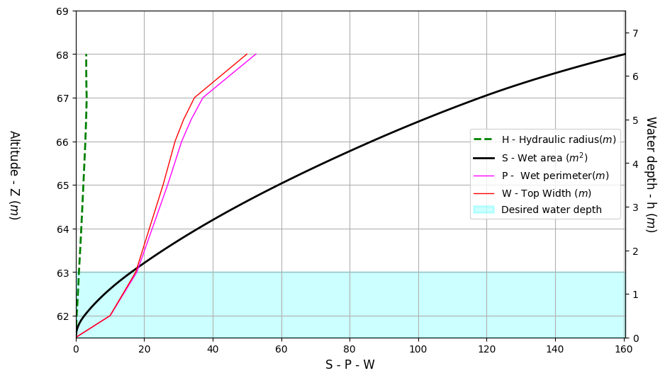
Plotting the relations
[13]:
fig, ax = plt.subplots(figsize=(10,6))
prof_small.plotcs_relations(show=True, fig=fig, ax=ax)
ax.legend()
D:\ProgrammationGitLab\HECEPython\docs\source\tutorials\../../..\wolfhece\PyCrosssections.py:2087: UserWarning: FigureCanvasAgg is non-interactive, and thus cannot be shown
  fig.show()
[13]:
<matplotlib.legend.Legend at 0x1936cfc5250>

We can add a specific position in terms of water depth…
[14]:
fig, ax = plt.subplots(figsize=(10,6))
prof_small.plotcs_relations(show=True, fig=fig, ax=ax,
                            fwd=1.5,  # desired water depth
                            )
ax.legend()
[14]:
<matplotlib.legend.Legend at 0x193711285d0>
… or water elevation !
[15]:
fig, ax = plt.subplots(figsize=(10,6))
prof_small.plotcs_relations(show=True, fig=fig, ax=ax,
                            fwl=64.2,  # desired water elevation
                            )
ax.legend()
[15]:
<matplotlib.legend.Legend at 0x193715efe10>

Add “banks” position
You can add banks elevations with the attributes leftbank and rightbank.
Position of the banks can be defined in three ways with the attribute banksbed_postype:
postype.BY_ELEVATION(default) : The banks are defined by their elevation.postype.BY_INDEX: The banks are defined by their index (0 based).postype.BY_S: The banks are defined by their curvilinear abscissa (0 based).
[16]:
from wolfhece.PyCrosssections import postype
prof_small.banksbed_postype = postype.BY_INDEX # We will define the banks by their index - 0 based

print("Number of points in the section: ", prof_small.nbvertices)

prof_small.bankleft = 1
prof_small.bankright = 8
prof_small.prepare() # We must prepare manually the profile after changing the banks (Not included in `bankleft` and `bankright` setters)
prof_small.plot_cs() # Left and right banks are shown on the plot
Number of points in the section: 11
[16]:
(-15.0, -100024.0, 15.0, 67.0, -99999.0, 66.0)

If defined, banks are added on the cross-section plot and on the relations plot.
[17]:
fig, ax = plt.subplots(figsize=(10,6))
prof_small.plotcs_relations(show=True, fig=fig, ax=ax,
                            fwl=64.2,  # desired water elevation
                            )
ax.legend()
[17]:
<matplotlib.legend.Legend at 0x193719048d0>

Add more positions - “bed”, “left_down”, “right_down”
Similar to banks, you can add more positions with the attributes:
bed: The lowest point of the section / riverbedleft_down: The left down point of the left bankright_down: The right down point of the right bank
[18]:
fig, ax = plt.subplots(figsize=(10,6))
prof_small.bankleft_down = 3
prof_small.bankright_down = 6
prof_small.bed = 5
prof_small.prepare() # We must prepare manually the profile after changing the banks (Not included in `bankleft` and `bankright` setters)
prof_small.plot_cs(fig=fig, ax = ax) # Left and right banks are shown on the plot
[18]:
(-15.0, -1.0, 15.0, 67.0, 61.5, 66.0)

Uniform Manning-Strickler Discharge / Water Depth
Computing the uniform water depth using the Manning-Strickler formula is an implicit process that requires solving a nonlinear equation. The Manning-Strickler formula is:
where:
$ Q $ is the discharge [m³/s]
$ n $ is the Manning roughness coefficient [$ s·m^{-1/3} $]
$ A $ is the wetted area [m²]
$ R $ is the hydraulic radius [m]
$ S $ is the slope [-] The Strickler coefficient $ K $ is the inverse of Manning’s $ n $: $ K = 1/n $ [$ m{1/3}·s{-1} $].
On the other hand, computing the uniform discharge for a given water depth is an explicit process. Therefore, it is easier to compute the discharge for a given water depth than to determine the water depth for a given discharge.
You can use the ManningStrickler_profile method to compute the uniform discharge for a given water depth. The results are stored in the q_slope attribute.
In this method, you must specify the slope (strictly positive), and either the Manning $ n $ or Strickler $ K $ coefficient. If both are provided, Manning’s $ n $ is used.
[19]:
prof_small.ManningStrickler_profile(slope = 2e-3, nManning = 0.03)
[19]:
np.float64(900.6624498251274)
You can plot the uniform AND critical discharge relation with the plot_discharges_UnCr method.
The relative position of each curve indicate the flow regime :
If the uniform discharge curve is above the critical discharge curve, the flow is “fluvial”.
If the uniform discharge curve is below the critical discharge curve, the flow is “torrential”.
[20]:
fig, ax = plt.subplots(figsize=(10,6))
prof_small.plot_discharges_UnCr(fig=fig, ax=ax, show=True)
ax.legend()
D:\ProgrammationGitLab\HECEPython\docs\source\tutorials\../../..\wolfhece\PyCrosssections.py:1950: UserWarning: FigureCanvasAgg is non-interactive, and thus cannot be shown
  fig.show()
[20]:
<matplotlib.legend.Legend at 0x19371533b90>

[21]:
prof_large.ManningStrickler_Q(KStrickler=30.)
prof_large.ManningStrickler_profile(slope=0.01, KStrickler=30.)
prof_large.plotcs_discharges(show=False)

A more complex cross-section
[22]:
myprof3=profile('Special profile', data_sect = example_diffsect1)
myprof3.plot_cs(fwl=5.5)
myprof3.relations()
myprof3.ManningStrickler_Q(KStrickler=30.)
myprof3.plot_discharges_UnCr(show=True)


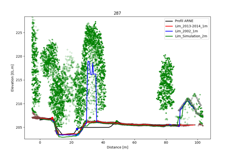
Compare the section with the tables and LAZ data.
If you have LAZ data, you can plot the cross-section with the points from the LAZ file located near the section.
The same applies to WolfArrays. The Z values are extracted at the array resolution in order to be compared with the profile discretisation.
Example of comparison: