Notebook: Creation of a 2D Modeling via Script - Short Version

To create a 2D simulation, it is necessary to:

create a “prev_sim2D” instance by providing the full path and the generic name of the simulation as an argument
define a vectorial contour/polygon delimiting the working area
(optional) define a “magnetic grid” used to snap the vertices of the polygons –> allows alignment between different models, for example
define the spatial resolution of the mesh on which the data (topography, friction, unknowns…) will initially be provided
define the contours/polygons of the blocks and their respective spatial resolution
call the mesher (call to the Fortran code)
create the mandatory matrices and fill them with the desired values (via script(s) or GUI)
create potential boundaries for boundary conditions (.sux, .suy)
impose the necessary boundary conditions (note: no conditions == impermeable)
configure the problem
execute the computation
process the results

Importing Modules

[11]:

import numpy as np
from tempfile import TemporaryDirectory
from pathlib import Path

from datetime import datetime as dt
from datetime import timezone as tz
from datetime import timedelta as td
from typing import Literal, Union

from wolfhece.mesh2d.wolf2dprev import prev_sim2D
from wolfhece.PyVertexvectors import zone, Zones, vector, wolfvertex
from wolfhece.wolf_array import WolfArray, WolfArrayMB
from wolfhece.wolfresults_2D import Wolfresults_2D, views_2D
from wolfhece.mesh2d.cst_2D_boundary_conditions import BCType_2D, Direction, revert_bc_type

Definition of the Working Directory

[12]:

outdir = Path(r'test')
outdir.mkdir(exist_ok=True) # Création du dossier de sortie
print(outdir.name)

test

Verification of the presence of the “wolfcli” code

Returns the full path to the code

[13]:

wolfcli = prev_sim2D.check_wolfcli() # méthode de classe, il n'est donc pas nécessaire d'instancier la classe pour l'appeler

if wolfcli:
    print('Code found : ', wolfcli)
else:
    print('Code not found !')

Code found :  C:\Users\pierre\Documents\Gitlab\Python310new\Lib\site-packages\wolfhece\libs\wolfcli.exe

Creation of a 2D simulation object

[14]:

# Passage en attribut du répertoire de travail auquel on a ajouté le nom générique de la simulation.
# "clear" permet de supprimer les fichiers de la simulation précédente.
newsim = prev_sim2D(fname=str(outdir / 'test'), clear=True)

# Un message de type "logging.info" est émis car aucun fichier n'a été trouvé. Ceci est normal !
# Si un fichier est trouvé, il est chargé.

WARNING:root:No infiltration file found

Geometry of the Problem

Definition of the external polygon – using a “vector” class – see wolfhece.PyVertexvectors

Square domain of size 1.0 m x 1.0 m

[15]:

# Define the extrenal contour
extern = vector()
extern.add_vertex(wolfvertex(0., 0.))
extern.add_vertex(wolfvertex(1., 0.))
extern.add_vertex(wolfvertex(1., 1.))
extern.add_vertex(wolfvertex(0., 1.))
extern.close_force()

print('Nombre de vertices : ', extern.nbvertices)
print('5 vertices car la polygone est fermé et le dernier point est aux mêmes coordonnées que le premier.')

Nombre de vertices :  5
5 vertices car la polygone est fermé et le dernier point est aux mêmes coordonnées que le premier.

Setup Steps

[16]:

# "Very Fast" - One block
# -----------------------

# # with tuple
# newsim.setup_oneblock((0.,0.,1,1,1.,1.), block_spatial_stepsize = 0.1, friction_coefficient =0.04)

# # with dictionary
# newsim.setup_oneblock({'ox': 0., 'oy': 0., 'nbx':1, 'nby':1, 'dx': 1., 'dy': 1.}, block_spatial_stepsize = 0.1, friction_coefficient = 0.04)

[ ]:

# More verbose - One block
# ------------------------

# Magnetic grid - dx and dy are the grid steps [m], origx and origy are the coordinates of the first point of the grid.
#   The magnetic grid has nothing to do with the spatial resolution of the calculation. It is used to move the contour points of the blocks to place them on the magnetic grid.
#   This ensures that the edges of the blocks will be perfectly aligned on the fine grid.
newsim.set_magnetic_grid(dx=1., dy=1., origx=0., origy=0.)

# Transfer the polygon as the external simulation boundary.
newsim.set_external_border_vector(extern)

# By default, the coordinates of the polygon will be translated so that the point (xmin, ymin) is at (0, 0).
newsim.translate_origin2zero = True

# Choice of the fine mesh spatial step size [m].
newsim.set_mesh_fine_size(dx=0.1, dy=0.1)

# Adding a block with its specific spatial step size [m].
newsim.add_block(extern, dx=0.2, dy=0.2)

# Meshing the problem
if newsim.mesh():
    print('Meshing done!')
else:
    print('Meshing failed!')

# If "with_turbulence" is True, the ".kbin" and ".epsbin" files will also be created and will contain the turbulent kinetic energy.
newsim.create_fine_arrays(default_frot=0.04, with_tubulence=False)

# Search for potential boundary conditions based on the ".napbin" matrix and write the ".sux" and ".suy" files.
newsim.create_sux_suy()

Meshing done !

At this stage, files should be present in your modeling directory.

We might wonder about the size of the “fine” matrices, i.e., the matrices with a resolution of 0.1m x 0.1m.

Given that the desired computational domain is 1.0m x 1.0m, the size is:

nbx = int(length_x / dx_fin) + 2 + 2 * 3 * (dx_block / dx_fin) = 10 + 2 + 6 = 18
nby = int(length_y / dy_fin) + 2 + 2 * 3 * (dy_block / dy_fin) = 10 + 2 + 6 = 18

Around the computational domain, there is 1 fringe cell all around (dx_fin, dy_fin) + 3 times the largest block cell size.

In this example, since there is only one block but its cell size is twice that of the fine matrix, there are 8 additional cells all around.

Thus:

The first computational cell is at position (5,5) with a 1-based convention, Fortran-style, or (4,4) with a 0-based convention, Python-style.
The last computational cell is at position (14,14) with a 1-based convention, Fortran-style, or (13,13) with a 0-based convention, Python-style.
The first X-oriented boundary is at index (5,5) with a 1-based convention, Fortran-style, or (4,4) with a 0-based convention, Python-style.
The first Y-oriented boundary is at index (5,5) with a 1-based convention, Fortran-style, or (4,4) with a 0-based convention, Python-style.
The last X-oriented boundary is at index (15,15) with a 1-based convention, Fortran-style, or (14,14) with a 0-based convention, Python-style.
The last Y-oriented boundary is at index (15,15) with a 1-based convention, Fortran-style, or (14,14) with a 0-based convention, Python-style.

[ ]:

print('Shape of the mesh : ', newsim.nbx, newsim.nby) # must be 18,18

Shape of the mesh :  18 18

[ ]:

assert newsim.napbin.array.data[4,4] == 1, 'napbin[4,4] should be 1'
assert newsim.napbin.array.data[3,3] == 0, 'napbin[3,3] should be 0'
assert newsim.napbin.array.data[newsim.nbx-4,newsim.nby-4] == 0, 'napbin[nbx-4,nby-4] should be 0'
assert newsim.napbin.array.data[newsim.nbx-5,newsim.nby-5] == 1, 'napbin[nbx-5,nby-5] should be 1'

assert newsim.napbin.array[3,3] is np.ma.masked, 'napbin[3,3] should be masked'

Parameters

[29]:

newsim.parameters.set_params_time_iterations(nb_timesteps= 1000, optimize_timestep=True, writing_frequency=1, writing_mode='Iterations', initial_cond_reading_mode='Binary', writing_type='Binary compressed')
newsim.parameters.set_params_temporal_scheme(RungeKutta='RK21', CourantNumber=0.35)

Checks

[30]:

# Plusieurs niveaux de vebrosité sont disponibles:
#   - 0 : Erreurs uniquement
#   - 1 : Erreurs et Warnings
#   - 2 : Erreurs, Warnings et Informations
#   - 3 : 2 + en-têtes de sections
print(newsim.check_all(verbosity= 0))

Boundary conditions

[ ]:

newsim.reset_all_boundary_conditions()

# ou via des boucles, tout est possible !
for j in range(5,15): # -> bouclage de 5 à 14 inclus
    newsim.add_boundary_condition(i = 15, j = j, bc_type = BCType_2D.H, bc_value = 1.0, border=Direction.X)

for j in range(5,15): # -> bouclage de 5 à 14 inclus
    newsim.add_boundary_condition(i = 5, j = j, bc_type = BCType_2D.QX, bc_value = 1.0, border=Direction.X)
    newsim.add_boundary_condition(i = 5, j = j, bc_type = BCType_2D.QY, bc_value = 0.0, border=Direction.X)

Listing of BCs along each axis:

Number of BCs
List the indices
Obtain a list of “boundary_condition_2D” objects - https://wolf.hece.uliege.be/autoapi/wolfgpu/simple_simulation/index.html#wolfgpu.simple_simulation.boundary_condition_2D
Check existence or not
Change the value and/or type
Remove a previously imposed condition

[34]:

print('Nb CL selon X : ', newsim.nb_weak_bc_x)
print('Nb CL selon Y : ', newsim.nb_weak_bc_y)

Nb CL selon X :  30
Nb CL selon Y :  0

Saving to Disk

Parameters and boundary conditions can be saved to disk in the “.par” file using the “save” method.

Writing to disk can therefore only be validly performed after defining both the necessary parameters and the problem’s boundary conditions.

[35]:

newsim.save()

WARNING:root:No infiltration data to write

Initial Conditions / Data

Topography

[36]:

# mise à zéro de la topographie
newsim.top.array[:,:] = 0.0

Initial water depth

[37]:

# Comme la topo est plate, on peut facilement éditer la matrice de hauteur d'eau
newsim.hbin.array[:,:] = 1.0

Unit discharges along X and Y

[38]:

newsim.qxbin.array[:,:] = 0.
newsim.qybin.array[:,:] = 0.

Friction coefficient

We keep the default value of 0.04

Saving

The matrices are referenced in the object.

We force the update of the files.

[39]:

newsim.save_arrays_modifications()

Calculation

Once all the files are written to disk, it is time to start the calculation.

To do this, either use “run_wolfcli” or execute the command “wolfcli run_wolf2d_prev genfile=pathtosim” in a command window, provided that wolfcli is accessible there (e.g., via the PATH).

[41]:

newsim.run_wolfcli()

Be Patient!!

The calculation is in progress… at least if a command window appears and calculation information is displayed.

The total calculation time is impossible to predict.

WARNING If a file access error is mentioned, it is likely related to another window still open or an unclosed file link. Start by closing all previous command windows and restart the script.

Results Analysis

[19]:

# Instanciation d'un objet résultat
res = Wolfresults_2D(newsim.filename)

[20]:

# Récupération du nombre de résultats
res.get_nbresults()

# 1001 car 1000 itérations + 1 état initial

[20]:

[21]:

# Récupération des résultats d'un pas spécifique (0-based) -- "-1" pour le dernier pas
res.read_oneresult(-1)

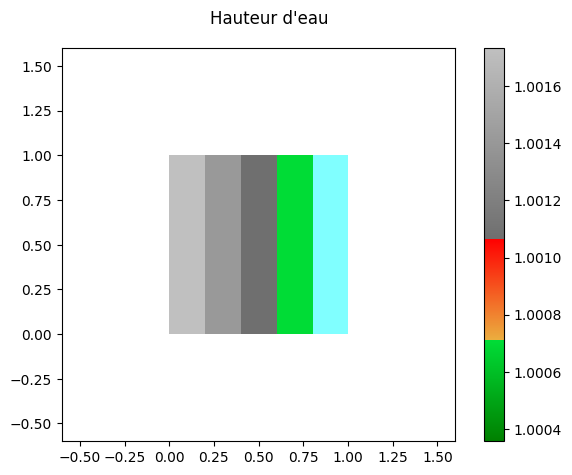
Simple Matplotlib Display of the Last Step

[22]:

res.read_oneresult(-1)
res.set_current(views_2D.WATERDEPTH) # Calcul de la hauteur d'eau

[23]:

print('Minimum ', res[0].array.min())
print('Maximum ', res[0].array.max())

fig,ax = res[0].plot_matplotlib()
fig.suptitle('Hauteur d\'eau')
fig.colorbar(ax.images[0], ax=ax)
fig.tight_layout()

Minimum  1.0003558
Maximum  1.0017345

../_images/2d_setup_sim2D_CPU_short_english_47_1.png

It might also be time to open the WOLF interface for more interactivity…