Mathematical model
The flow model is based on the two-dimensional depth-averaged equations of volume and momentum conservation. In the “shallow-water” approach, it is basically assumed that velocities normal to the main flow plane are significantly smaller than those in this main flow direction. Consequently, the pressure field is almost hydrostatic everywhere.
The large majority of flows occurring in rivers, even highly transient, can reasonably be seen as shallow everywhere, except in the vicinity of some singularities (e.g. weirs). Indeed, vertical velocity components remain generally low compared to velocity components in the horizontal plane and, consequently, flows may be considered as mainly two-dimensional. Thus, the approach used in WOLF is suitable for many of the problems encountered in river management, and especially flood inundation mapping.
The conservative form of the depth-averaged equations of volume and momentum conservation can be written as follows, using vector notations:
where \({\bf{s}} = {\left[ {\begin{array}{\*{20}{c}} h&{hu}&{hv} \end{array}} \right]^{\rm{T}}}\) is the vector of the conservative unknowns. \(\bf{f}\) and \(\bf{g}\) represent the advective and pressure fluxes in directions \(x\) and \(y\), while \({\bf{f}}_{\rm{d}}\) and \({\bf{g}}_{\rm{d}}\) are the diffusive fluxes:
\({\bf{S}}_0\) and \({\bf{S}}_f\) designate respectively the bottom slope and the friction terms:
In Eq. (1) to (7), \(t\) is the time, \(x\) and \(y\) the space coordinates, \(h\) the water depth, \(ut\) and \(v\) the depth-averaged velocity components, \(z_b\) the bottom elevation, \(g\) the gravity acceleration, \(\rho\) the density of water, \(\tau _{bx}\) and \(\tau _{by}\) the bottom shear stresses, \(\sigma _x\) and \(\sigma _y\) the turbulent normal stresses, and \(\tau _{xy}\) the turbulent shear stress. Consistently with Hervouet (2003),
can reproduce the increased friction area on an irregular (natural) topography (Dewals, 2006).
Friction modelling
The bottom friction is conventionally modelled with empirical laws, such as the Manning formula. The model enables the definition of a spatially distributed roughness coefficient to impact different land-uses, floodplain vegetations or sub-grid bed forms… In addition, the friction along side walls is reproduced through a process-oriented formulation developed by Dewals (2006). Finally, friction terms become:
and
where the Manning coefficient \({n_{\rm{b}}}\) and \({n_{\rm{w}}}\) characterize respectively the bottom and the side-walls roughness. These relations have been written for Cartesian grids, such as used in the present study.
The internal friction might be reproduced by applying a proper turbulence model. For SWE, various approaches are proposed in the literature, as rather simple algebraic expressions of turbulent viscosity (Fisher et al., 1979; Hervouet, 2003) or more complex mathematical models with 1 or 2 additional equations (Rastogi and Rodi, 1978; Rodi, 1984; Erpicum, 2006).
In WOLF2D, there are several formulations available to compute the turbulent shear stresses. The simplest one is the mixing length model with a constant turbulent viscosity. The most complex one is an original 2D k-epsilon model (Erpicum, 2006).
The bottom friction models available in WOLF2D (Fortran) are :
Manning/Strickler
Barr-Bathurst
Colebrrok-White (fully semi-implicit or explicit)
Bazin
Haaland
Hazen-Williams
Grid and numerical scheme
The solver includes a mesh generator and can deal with multiblock grids (Erpicum, 2006). Within each block, the grid is Cartesian to take advantage of the lower computation time and the gain in accuracy provided by this type of structured grids compared to unstructured ones.
The multiblock features increase the domain area which can be discretized with a constant cells number and enable local mesh refinements close to areas of interest. It is thus a solution to overcome the main drawback of Cartesian grid, i.e. the high number of cells needed for a fine enough discretization of complexes geometries. Moreover, it allows combining local high precision with strong computation speed requirements.
In addition, an automatic grid adaptation technique restricts the simulation domain to the wet cells to decrease the number of computational elements. An original iterative technique restores mass and momentum conservation at each step of meshes drying.
Eq. (1) is discretized in space with a finite volume scheme. This ensures a correct mass and momentum conservation, which is a must for handling properly discontinuous solutions such as moving hydraulic jumps. As a consequence, no assumption is required regarding the smoothness of the solution. Reconstruction at cells interfaces can be performed with a constant or linear approach. For the latter, together with slope limiting, a second-order spatial accuracy is obtained.
In a similar way, variables at the border between adjacent blocks are reconstructed linearly, using in addition ghost points as depicted in Fig. 1. The value of the variables at the ghost points is evaluated from the value of the subjacent cells. Moreover, to ensure conservation properties at the border between adjacent blocks and thus to compute accurate volume and momentum balances, fluxes related to the larger cells are computed at the level of the finer ones.
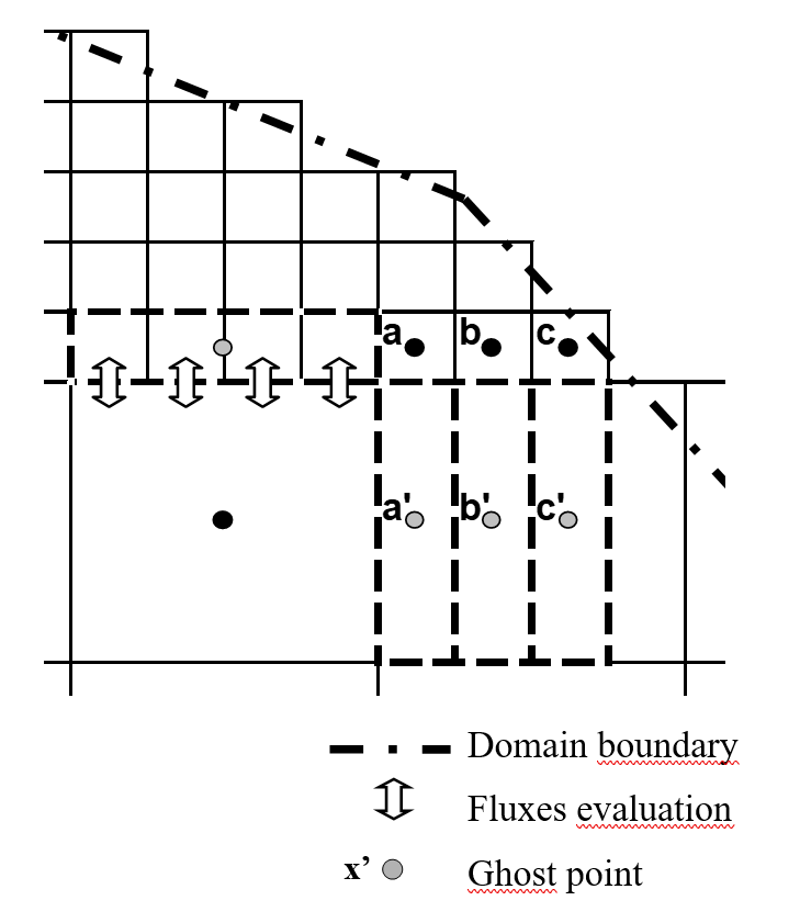
Fig. 1. Border between two adjacent blocks on a Cartesian multiblock grid – Ghost points for the reconstruction of the variables
Appropriate flux computation has always been a challenging issue in computational fluid dynamics. The fluxes \(\bf{f}\) and \(\bf{g}\) are computed by a Flux Vector Splitting (FVS) method, where the upwinding direction of each term of the fluxes is simply dictated by the sign of the flow velocity reconstructed at the cells interfaces. It can be formally expressed as:
where the exponents \(+\) and \(-\) refer to, respectively, an upstream and a downstream evaluation of the corresponding terms. A Von Neumann stability analysis has shown that this FVS ensures a stable spatial discretization of the terms \({\frac{\partial {\bf{f}}} {\partial x}}\) and \({\frac{\partial {\bf{g}}} {\partial y}}\) in Eq. (1) (Archambeau, 2006). Due to their diffusive character, the fluxes \({{\bf{f}}_{\rm{d}}}\) and \({{\bf{g}}_{\rm{d}}}\) can be determined by means of a centred scheme.
Besides low computation costs, this FVS has the advantages of being completely Froude independent and of facilitating the adequacy of discretization of the bottom slope term (Dewals et al., 2006; Dewals et al., 2008a, Archambeau, 2006).
Topography gradients
The discretization of the topography gradients is always a challenging task when setting up a numerical flow solver based on the SWE. The bed slope appears as a source term in the momentum equations. As a driving force of the flow, it has however to be discretized carefully, in particular regarding the treatment of the advective terms leading to the water movement, such as pressure and momentum.
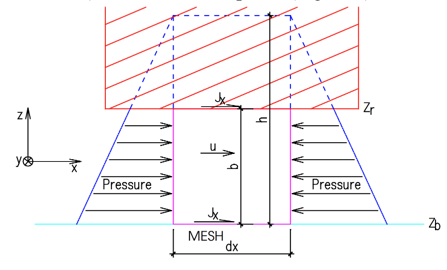
The first step to assess topography gradients discretization is to analyse the situation of still water on an irregular bottom. In this case, momentum equations simplify and there are only two remaining terms: the advective term of hydrostatic pressure variation and the topography gradient. For example, regarding x-axis equation
The hydrostatic pressure gradient has to be exactly counterbalanced by the bottom slope term. Analytically, the equation can be written as
with \(Z\) the free surface elevation. In case of water at rest, the free surface gradient is equal to zero and thus the free surface is horizontal.
In this case, assuming the bottom elevation and the water height are reconstructed coherently at the finite volume sides and their gradients are identically evaluated (Fig. 2), Eq. (12) can be written as
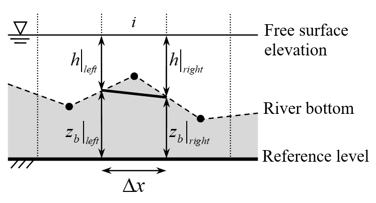
Fig. 2. Correspondence between the gradients of bottom elevation and water depth for water at rest
The space discretization has to provide equivalent conservative and non conservative forms of the pressure gradient. According to the FVS characteristics, a suitable treatment of the topography gradient source term of Eq. 6 is thus a downstream discretization of the bottom slope and a mean evaluation of the corresponding water depths (Erpicum, 2006). For a mesh \(i\) and considering a constant reconstruction of the variables, the bottom slope discretization writes:
where subscript \(i + 1\) refers to the downstream mesh along x-axis.
This approach fulfils the numerical compatibility conditions defined by Nujic (1995) regarding the stability of water at rest. The final formulation is the same as the one proposed by Soares (2000) or Audusse (2004).
The formulation is suited to be used in both 1- and 2D models, along x- and y- axis. Its very light expression benefits directly from the simplicity of the original spatial discretization scheme.
Nevertheless, the formulation of Eq. (18) constitutes only a first step towards an adequate form of the topography gradient as it is not entirely suited regarding water in movement over an irregular bed. The effect of kinetic terms is not taken into account and, consequently, poor evaluation of the flow energy evolution can occur when modeling flow, even stationary, over an irregular topography (Erpicum, 2006, Bruwier, 2016).
Time discretization
Since the model is applied to compute (highly) unsteady and/or steady-state solutions, the time integration is performed by means of an explicit Runge-Kutta scheme at various number of time steps.
1-step (Euler explicit) first order accurate
2-step second order accurate – used for transient computations.
3-step first order accurate – providing adequate dissipation in time is valuable for steady-state.
For stability reasons, the time step is constrained by the Courant-Friedrichs-Levy condition based on gravity waves. The time step is thus computed as:
where NC is the Courant number prescribed by the user. The stable value is depending on the Runge-Kutta algorithm used and the local hydrodynamics, but is lower than 1.
A semi-implicit treatment of the bottom friction term is used, without requiring additional computational costs.
Slight changes in the Runge-Kutta algorithm coefficients allow modifying its dissipation properties and make it suitable for accurate transient computations.
Boundary conditions (external or internal)
For each application, the value of the specific discharge can be prescribed as an inflow boundary condition. The transverse specific discharge is usually set to zero at the inflow even if a different value can be used if necessary. In case of supercritical flow, a water elevation can be provided as additional inflow boundary condition.
The inflow boundary conditions can be replaced by infiltration/exfiltration zones. In this case, certain cells are identified in the infiltration array, and the solver computes source terms (mass and momentum) based on the infiltration/exfiltration rate. Multiple infiltration/exfiltration zones can be defined for each model. It is possible to link some of these zones and compute the rate from Bernoulli’s equation based on the local head difference at each time step.
The outflow boundary condition may be a water surface elevation, a Froude number or no specific condition if the outflow is supercritical.
At solid walls, the component of the specific discharge normal to the wall is set to zero.
Topography data
Since 2000, high resolution, high accuracy topographic datasets have become increasingly available for inundation modelling in a number of countries. In Belgium, a data collection programme using airborne laser altimetry (LIDAR) has generated high quality topographic data covering the floodplains of most rivers in the southern part of the country (2002), the whole Region (2013-2014, 2021-2022) and more recently a combined data including bathymetry using green Lidar.
Wolf is very well suited to handle these high resolution datasets.
Methodology for systematic inundation mapping
Following a Regional Government decision in 2003, the solver WOLF2D, has been chosen to be used to compute a part of the official inundation hazard maps on 800 km of the main rivers of the Walloon Region in Belgium. This work has been performed in the scope of flood risk management, insurance of this risk, critical areas identification and climate change effects mitigation policy.
A 4-step modelling procedure has been elaborated and applied systematically for each river reach:
Elaboration from laser altimetry and sonar data (or cross sections) of the complete DEM (main riverbed and floodplains) with a grid resolution of 1 m by 1 m,
Validation and enhancement of the DEM by a field survey and the integration of additional geometric characteristics,
Flow modelling of past flood events with the purpose of calibrating and validating the roughness parameters,
Computation of the inundation maps for constant statistical flood discharge values (25-, 50- and 100-year return period and more if necessary).
Depending on the river width, steps 2 to 4 are conducted with a grid spacing varying between 1 m and 5 m, with a typical value of 2 m.
Now, we can deal with native 50 cm resolution data on quite large area using GPU computing.
The use of constant discharges to assess the consequences of flooding is justified by the morphology of the rivers studied. Indeed, as detailed by de Wit et al. (2007), the Meuse basin covers an area of about 33,000 km2, including parts of France, Luxembourg, Belgium, Germany and the Netherlands. It can be subdivided into three major geological zones, referred to as “Lotharingian Meuse” (southern part), “Ardennes Meuse” (central part) and the Dutch and Flemish lowlands (northern part).
While the southern and northern parts are characterized by wide floodplains where flood waves are significantly attenuated, in the central part of the Meuse basin, between Charleville-Mézières and Liège, the Meuse is captured in the Ardennes massif, characterized by narrow steep valleys, where flood waves are hardly attenuated.
For instance, for typical floods occurring on the river Ourthe, it has been verified that the volume of water stored in the inundated floodplains along a 10 km-long reach remains lower than one percent of the total amount of water brought by the flood wave.
Therefore, the steady-state assumption has been considered as valid for simulating floodplain inundation along most rivers of the Ardennes Massif.
However, the model natively computes flow in transient mode, including reaching a steady state. It is therefore possible to calculate any flood hydrograph (natural or artificial, like dike breaching or dam break).
Mixed flows, bridges and culverts
Note
Mainly based on the work of :
An exact Riemann solver and a Godunov scheme for simulating highly transient mixed flows, Kerger and al., Journal of Computational and Applied Mathematics, 2011, https://orbi.uliege.be/bitstream/2268/4272/1/Kerger_2011.pdf
1D unified mathematical model for environmental flow applied to steady aerated mixed flows, Kergerat al.. 2011 In Advances in Engineering Software, 42 (9), p. 660-670
EXPERIMENTAL INVESTIGATIONS OF 2D STATIONARY MIXED FLOWS AND NUMERICAL COMPARISON, Nam and al., https://orbi.uliege.be/bitstream/2268/129042/1/Fullpaper-Nam.pdf, IAHR, 2012
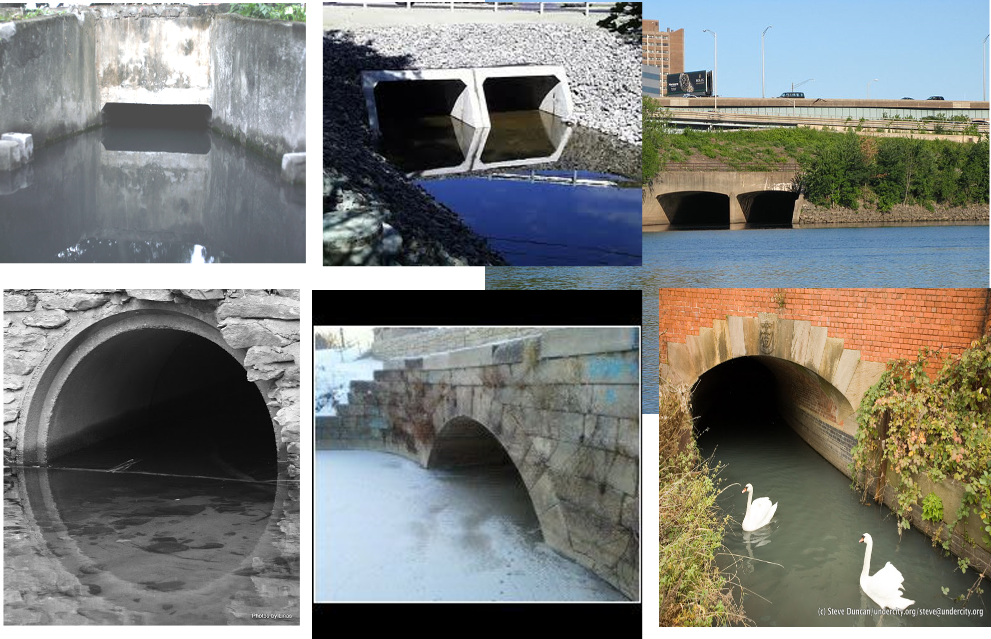
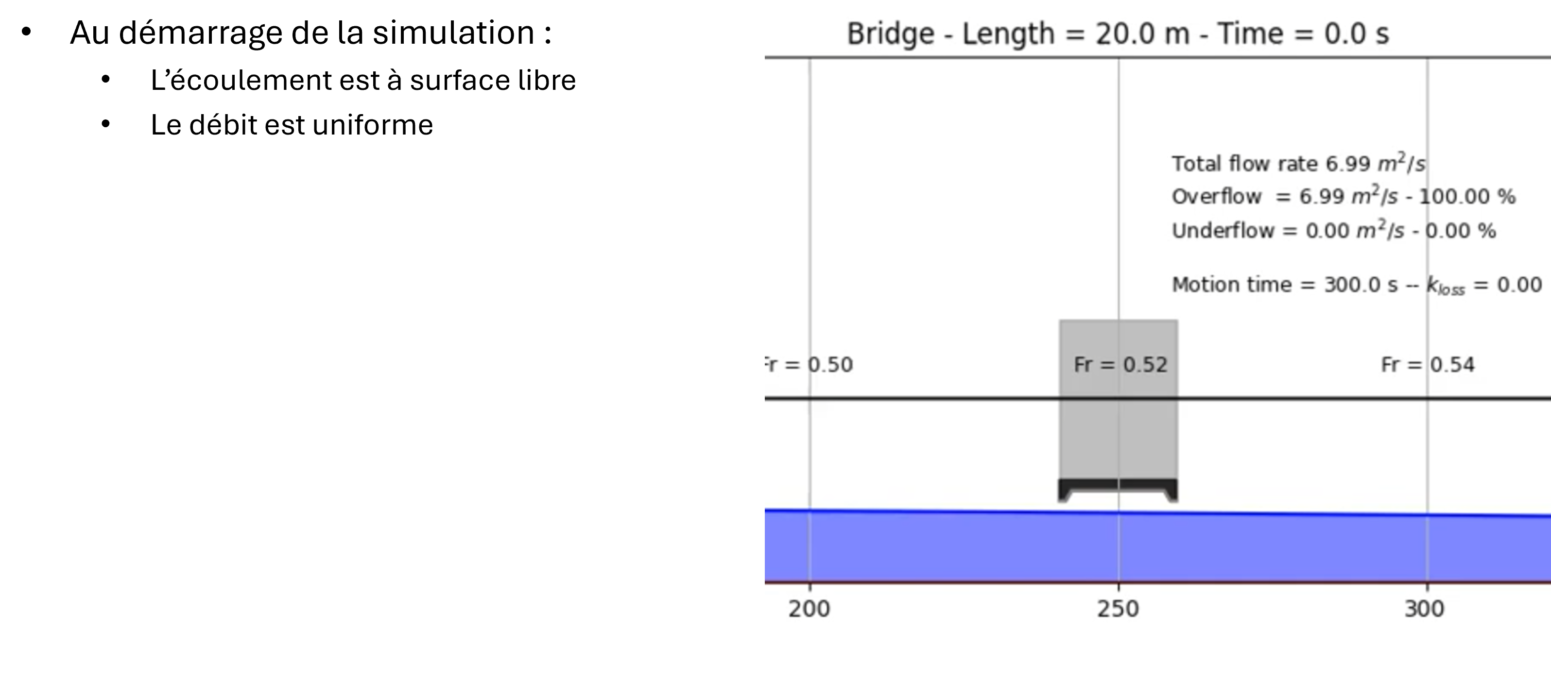
Mixed flows are known as the simultaneous occurrence of free-surface and pressurized flows. These phenomena are often encountered in water supply systems, sewer systems, storm-water storage pipes, flushing galleries, water conservancy projects, hydraulic structures, etc.. (Erpicum et al., 2008; Kerger et al., 2009).
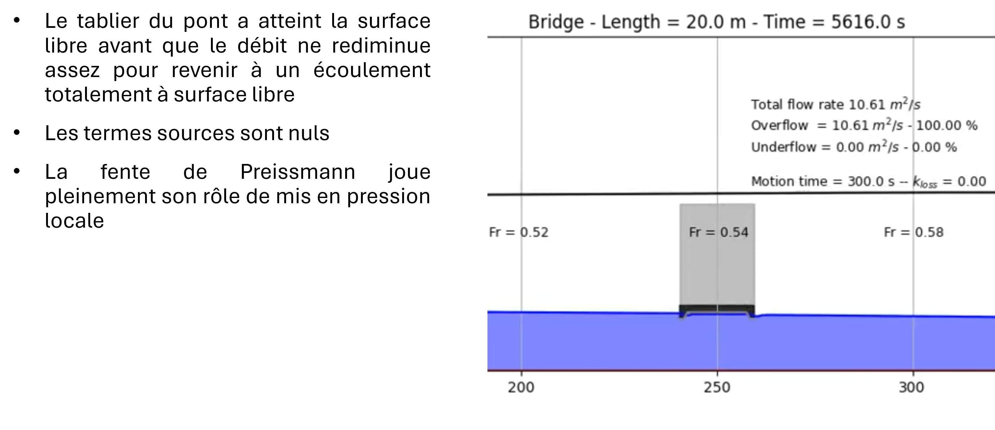
Using the Preissmann slot model (Preismann, 1961), pressurized flow can equally be calculated by means of the Saint-Venant equations by adding a conceptual slot on the top of a closed pipe. When the water level is above the maximum level of the cross-section, it provides a conceptual free surface flow, for which the gravity wave speed is related to the slot geometry (Kerger et al, 2009). The Preismann slot dimensions are the mesh size as in steady flow, pressure is not related to the slot characteristics.
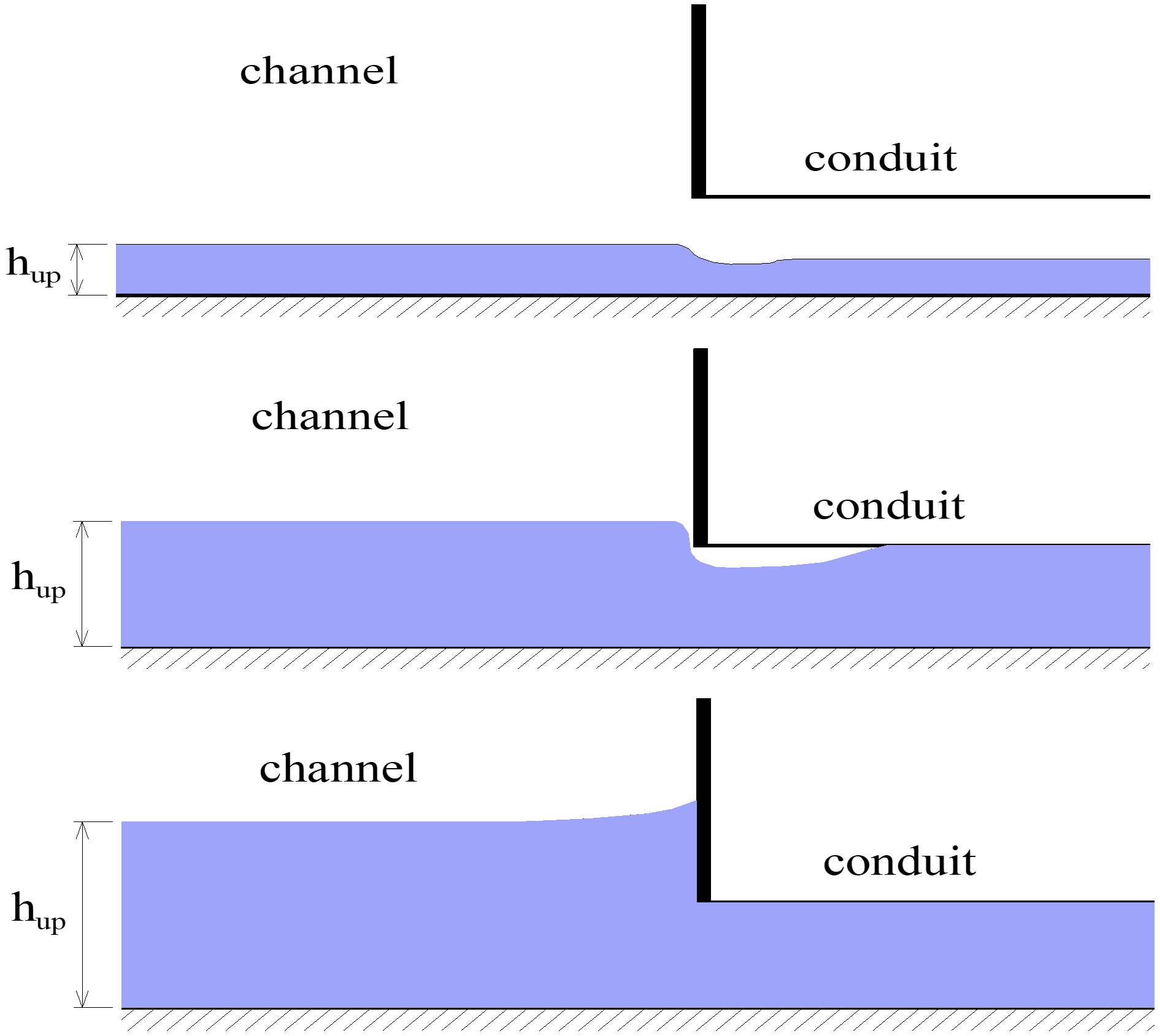
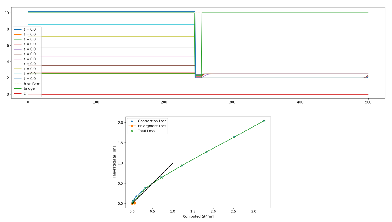
First example of a bridge with no overtopping. Ther flow is steady. Different discharge values are used to compute the flow with a fixed downstream boundary condition.
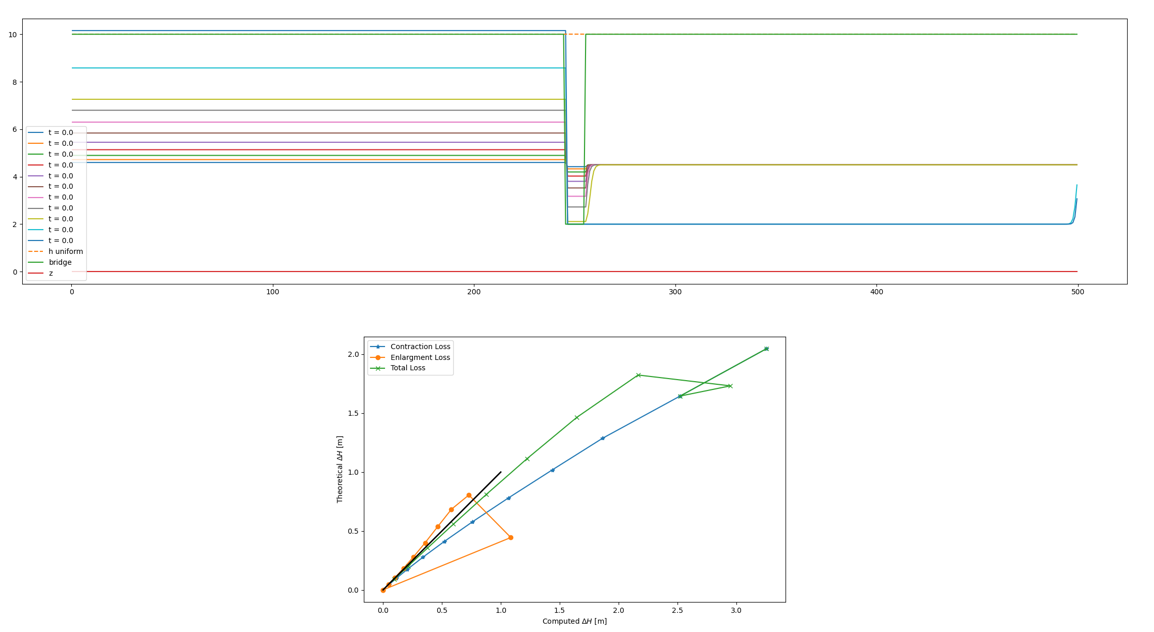
Second example of a bridge with no overtopping. Ther flow is steady. Different discharge values are used to compute the flow with a fixed downstream boundary condition.
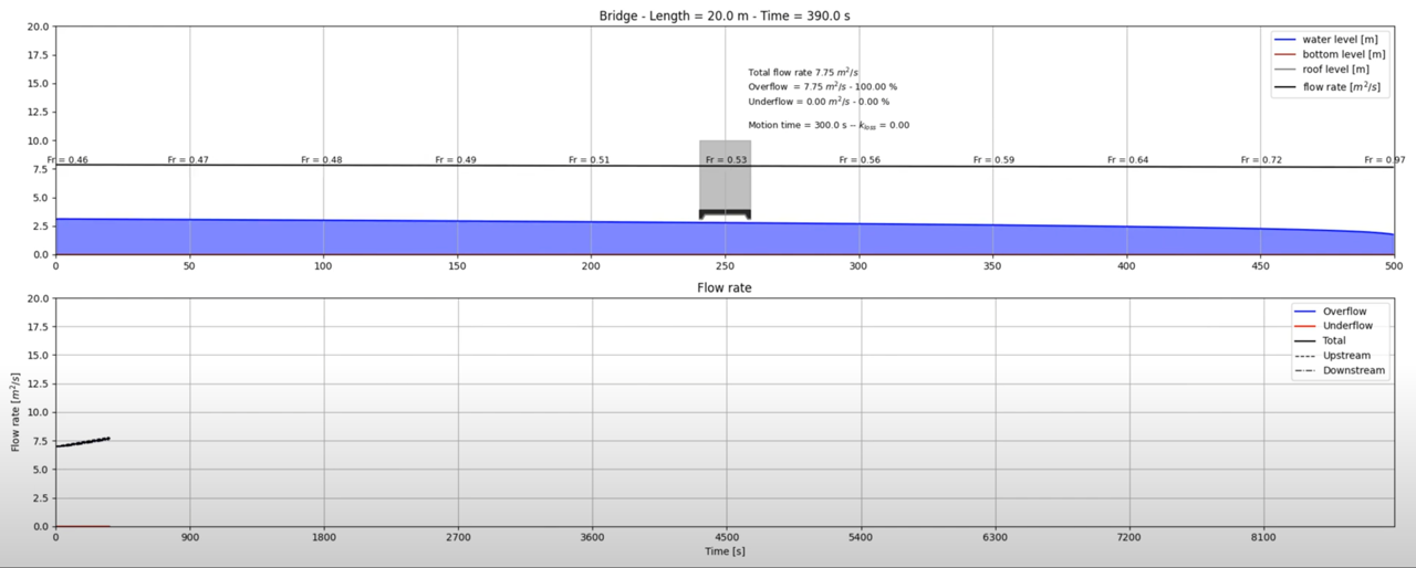
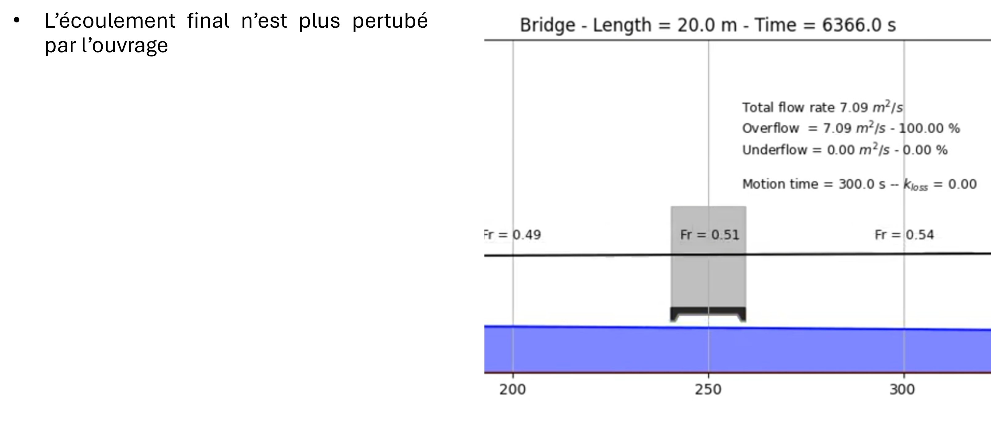
Third example of a bridge with no overtopping. Ther flow is unsteady. The discharge value is constant but the downstream boundary condition evolves (every 300 seconds).

There is a comparison between the head losses calculated by the code and the analytical formulation of local losses associated with contraction and expansion.
Overflows, bridges and culverts
In the same cell, modelling combined free-surface and pressurized flows is a challenging task using shallow-water equations.
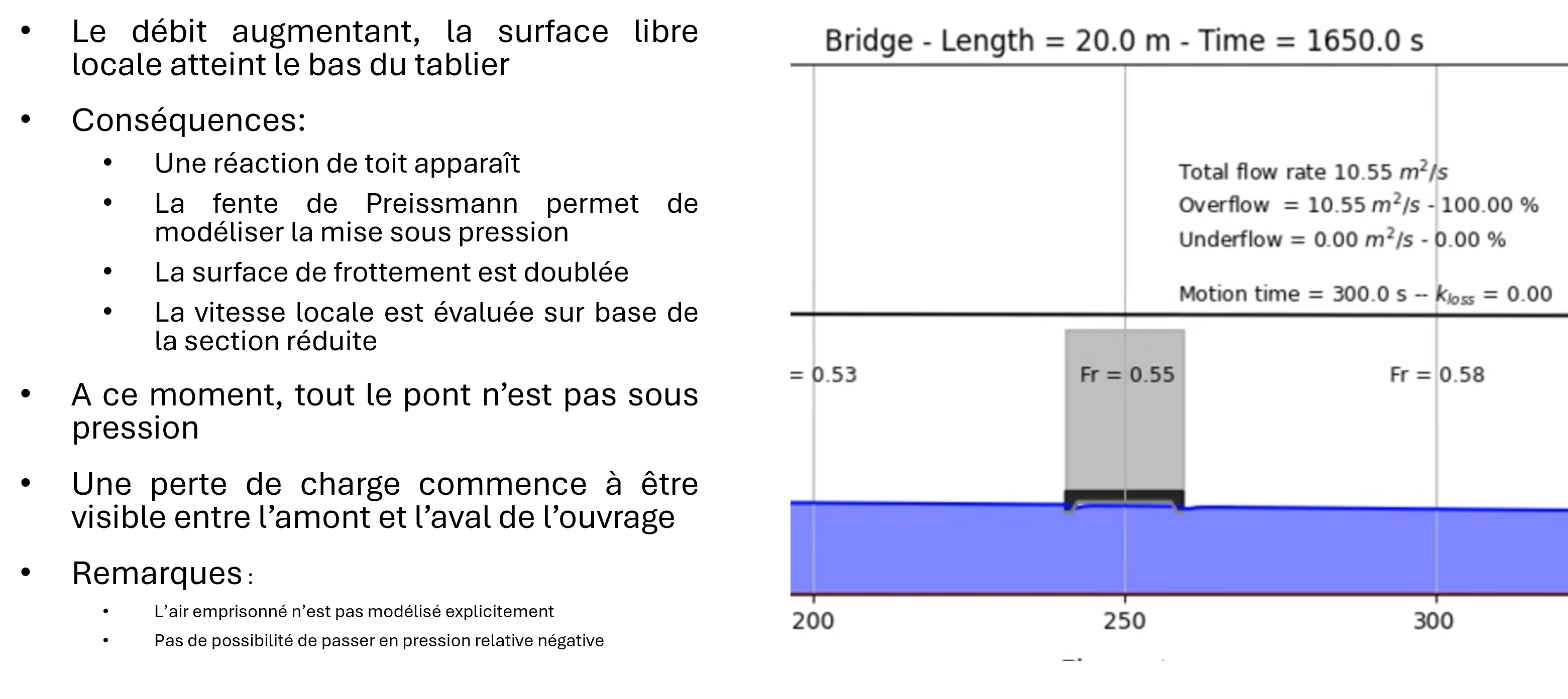
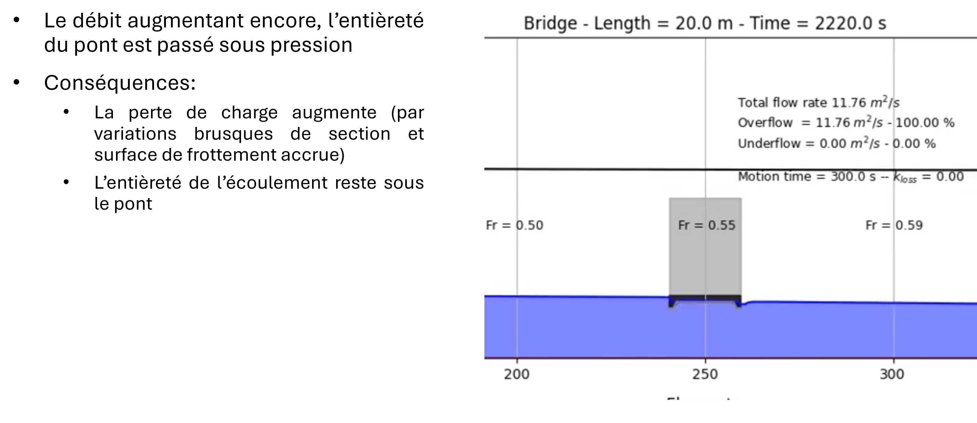
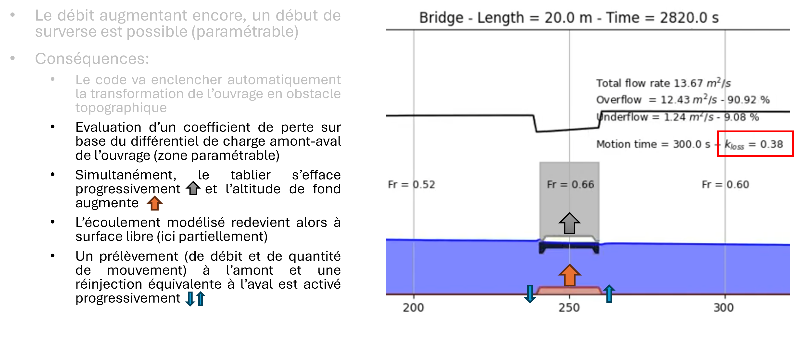
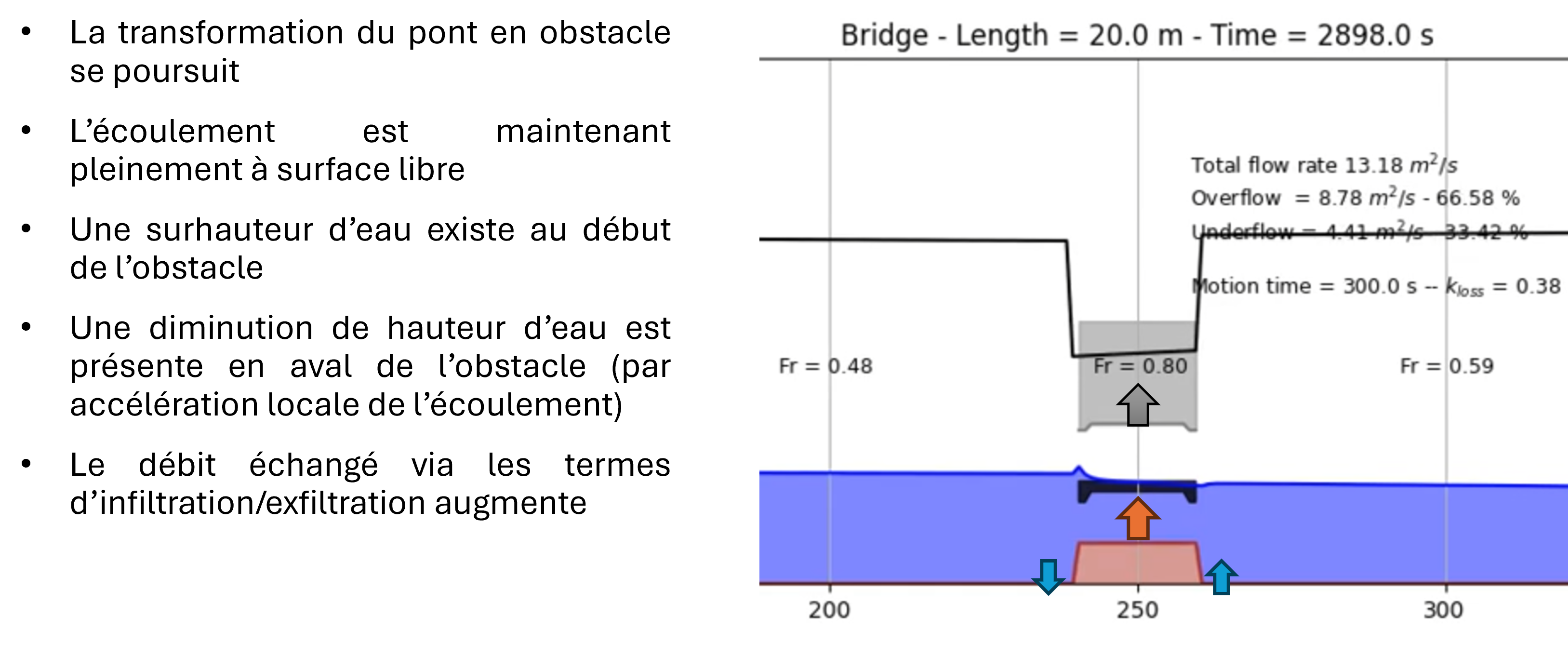
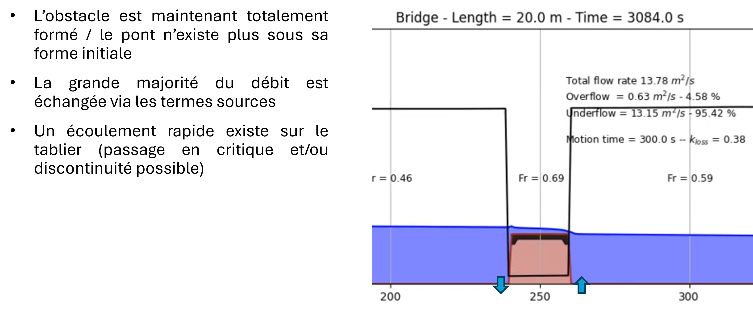
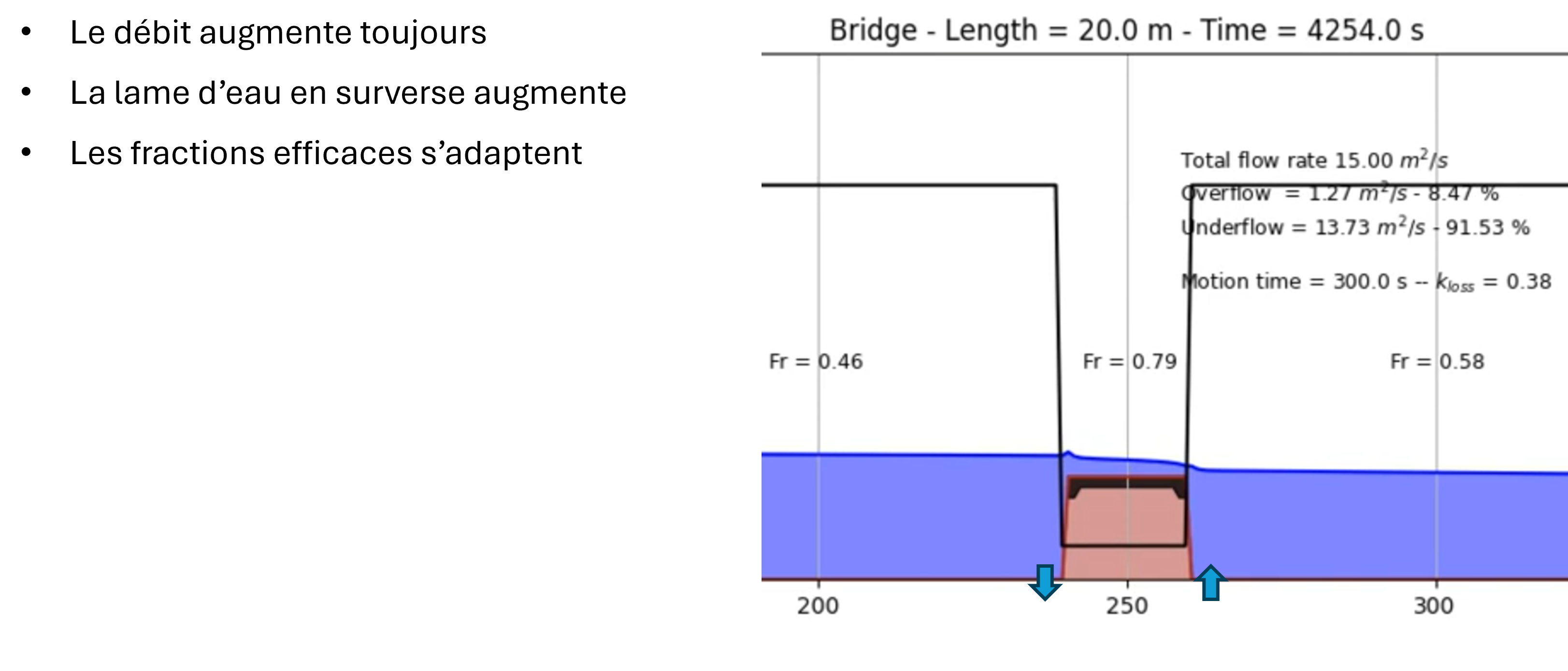
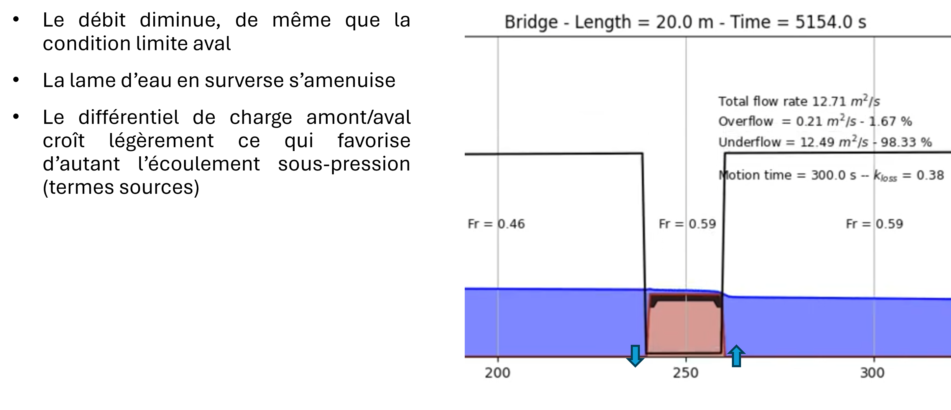
The solver is able of handling this type of flow by dynamically adapting the topography once the overflow criterion is reached. In this situation, after automatically estimating a head loss coefficient, the model progressively activates source terms (withdrawal upstream and restitution downstream of the structure) to simulate the effect of pressurized flow. The source terms are present in both the continuity and momentum equations.
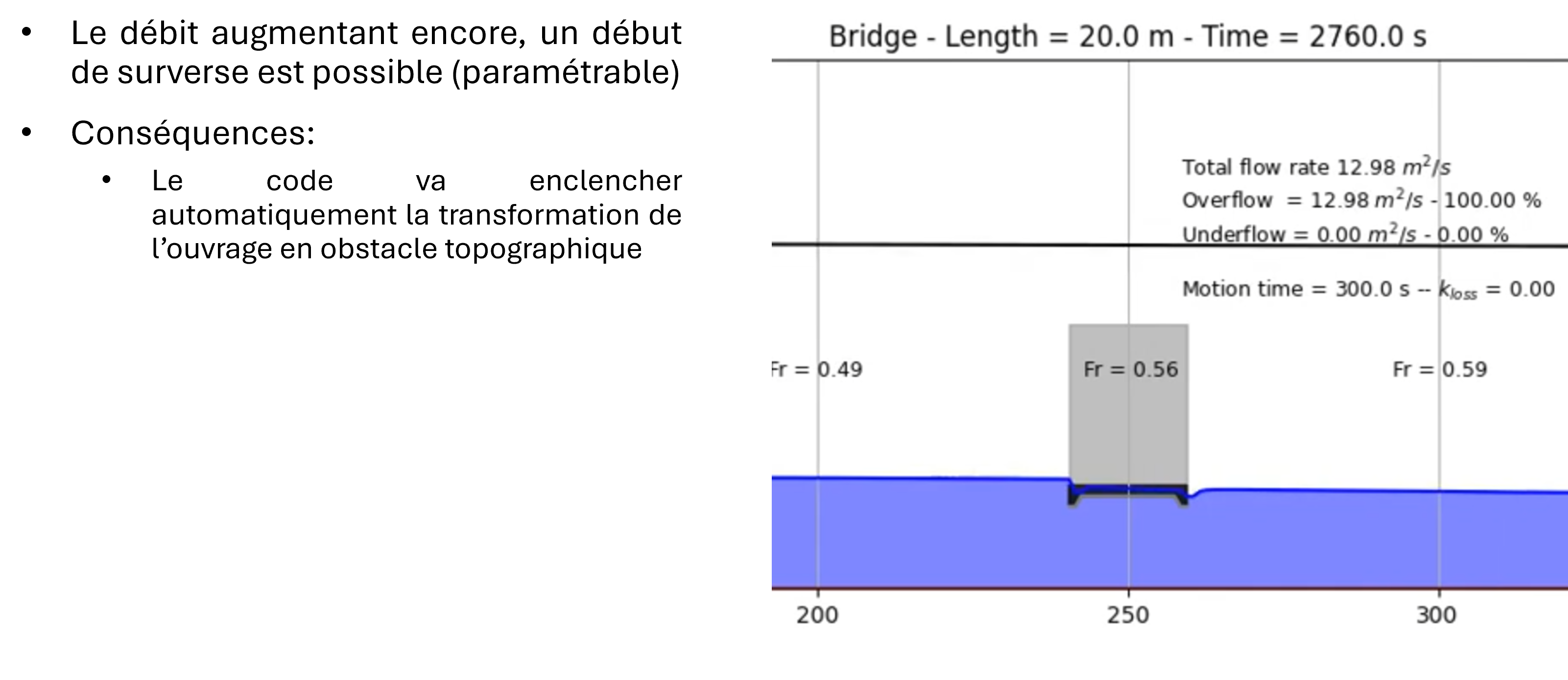
The altimetries (of the bottom and the roof of the structure) evolve simultaneously to transform the structure into an obstacle and allow overflow. During this phase, the lower discharge is evaluated based on the instantaneous head differential and is updated using the predetermined loss coefficient in the generalized Bernoulli equation (with temporal inertia).
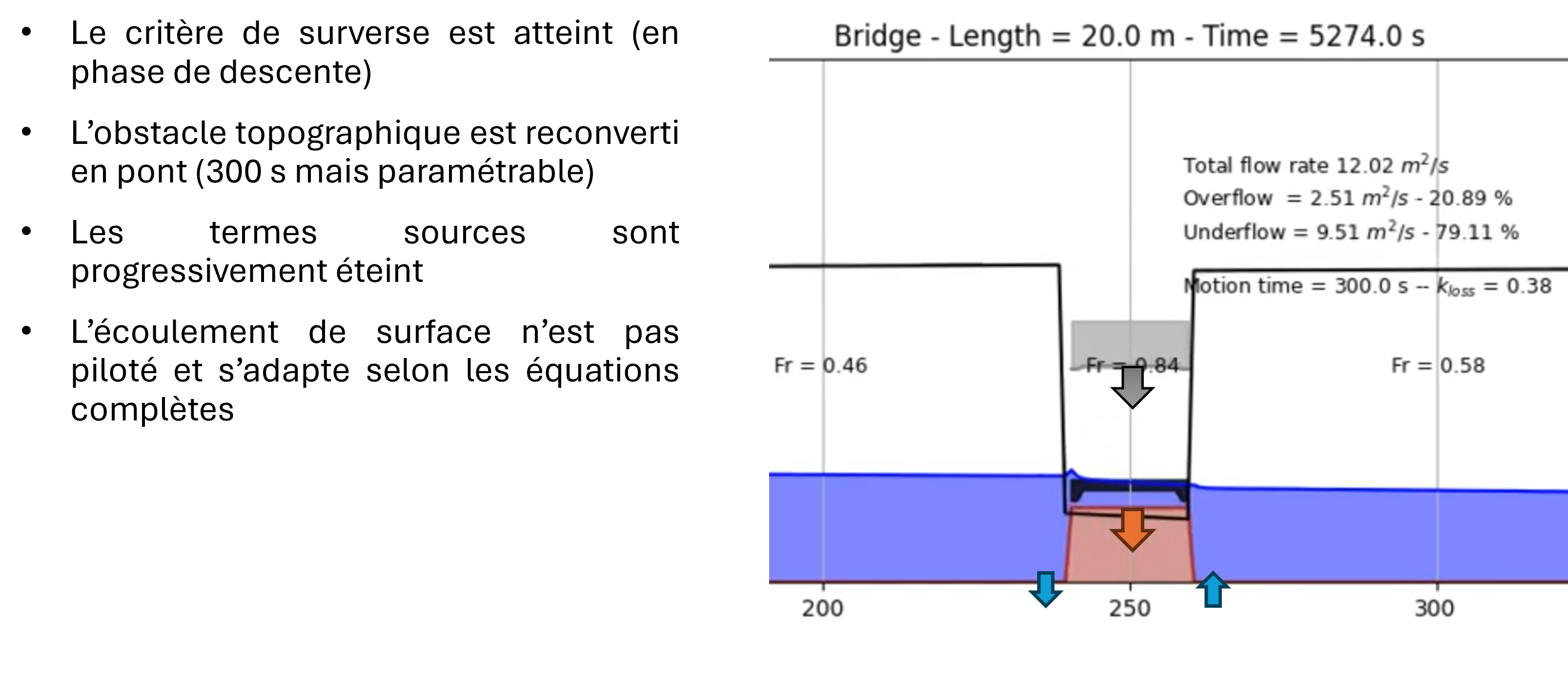
No assumption is made about the surface flow. It is therefore free to find a critical flow or not depending on the downstream submergence conditions.
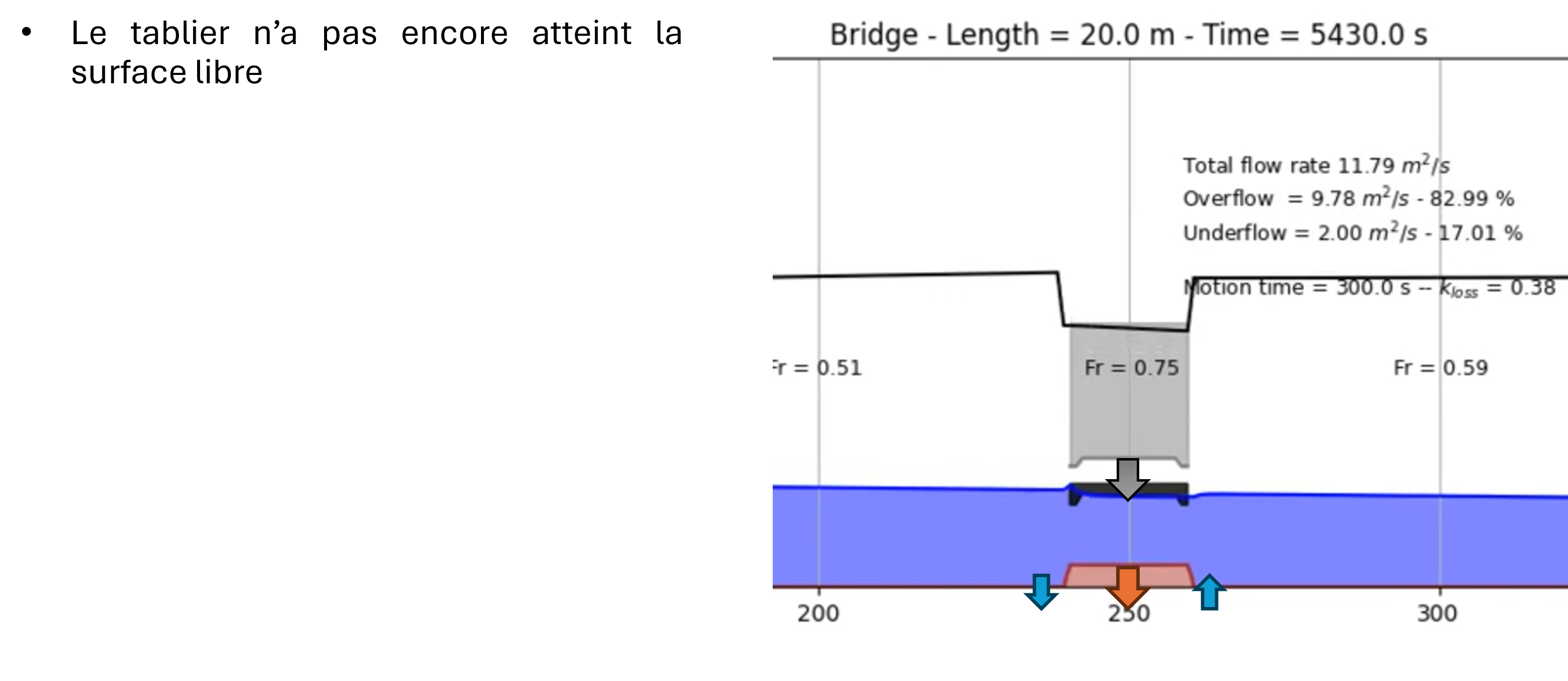
Once the structure is no longer submerged, the altimetries return to their initial shape and the flow becomes entirely free to either remain locally pressurized or revert to free surface flow everywhere.
- The available parameters are:
the motion time of the structure into an obstacle (in seconds)
the overflow detection criterion (altimetry in meters)
the local altimetry of the roof and deck of the structure (in meters)
the position of the source terms
the position of the head evaluation (upstream and downstream)
Note
- Main characteristics of the simulations:
Domain length: 500 m
Mesh size: 1 m
- Boundary conditions:
upstream: variable discharge
downstream: variable water height
Courant number: 0.4
Motion time: 300 seconds
Overflow detection criterion: 25 cm above the deck
Infiltration position: cell just upstream of the structure
Exfiltration position: cell just downstream of the structure
Head evaluation position: one cell offset from infiltration/exfiltration to correctly evaluate the kinetic energy/head component
Total simulation time: 9000 seconds
Bridge/culvert section: imposed by the user via local altimetries (V-shape, U-shape, rectangular shape…)
Bridge - V shape - Length : 20 m
Bridge - rectangular shape - Length : 20 m
Bridge - U shape - Length : 20 m
Culvert - Length : 100 m
Bridge - V shape - Length : 20 m - hydrograph + evolving downstream BC
Bridge - U shape - Length : 20 m - hydrograph + evolving downstream BC
Bridge - rectangular shape - Length : 20 m - hydrograph + evolving downstream BC
Bridge - rectangular shape - Length : 20 m - unsteady downstream boundary condition
Bridge - V shape - Length : 20 m - unsteady downstream boundary condition
Bridge - U shape - Length : 20 m - unsteady downstream boundary condition