WolfArray — Spatial Analysis

Note — All operations shown here work identically on WolfArrayModel (no GUI dependency). See the Model/GUI architecture tutorial for details.

This tutorial covers spatial analysis operations on WolfArray:

• Raster algebra (combining arrays with arithmetic operators)

• Masking chains (value-based and geometry-based)

• Resampling / rebinning with different aggregation operators

• Gradient / slope computation

• Spatial statistics

from wolfhece.wolf_array import WolfArray, header_wolf
import numpy as np
import matplotlib.pyplot as plt

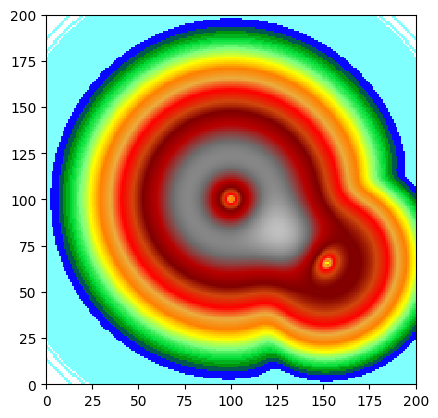
Setup: Synthetic DEM

h = header_wolf()
h.shape = (200, 200)
h.set_resolution(1., 1.)
h.set_origin(0., 0.)

dem = WolfArray(srcheader=h)

# Gaussian hill + valley
x = np.linspace(-3, 3, 200)
y = np.linspace(-3, 3, 200)
X, Y = np.meshgrid(x, y, indexing='ij')
dem.array[:, :] = 100. + 30. * np.exp(-(X**2 + Y**2)) - 10. * np.exp(-((X-1.5)**2 + (Y+1)**2)/0.5)

dem.plot_matplotlib(first_mask_data=False)

(<Figure size 640x480 with 1 Axes>, <Axes: >)

Raster Algebra

WolfArray supports full arithmetic: +, -, *, /, **, //, unary -, abs().

Operations are element-wise and produce a new WolfArray.

# Compute deviation from mean
mean_val = float(dem.statistics()['Mean'])
deviation = dem - mean_val      # scalar subtraction → new WolfArray
deviation.plot_matplotlib(first_mask_data=False)
print(f"Mean of deviation: {deviation.statistics()['Mean']:.6f} (≈0)")

INFO:root:No selection -- statistics on the whole array
INFO:root:No selection -- statistics on the whole array

Mean of deviation: -0.000005 (≈0)

# Normalise to [0, 1]
stats = dem.statistics()
vmin, vmax = float(stats['Min']), float(stats['Max'])
normalised = (dem - vmin) / (vmax - vmin)
print(f"Range: {normalised.statistics()['Min']:.4f} – {normalised.statistics()['Max']:.4f}")
normalised.plot_matplotlib(first_mask_data=False)

INFO:root:No selection -- statistics on the whole array
INFO:root:No selection -- statistics on the whole array
INFO:root:No selection -- statistics on the whole array

Range: 0.0000 – 1.0000

(<Figure size 640x480 with 1 Axes>, <Axes: >)

Masking Chains

Multiple mask operations can be chained to isolate specific regions by value.

# Isolate elevations between 105 and 120
band = WolfArray(mold=dem)
band.mask_lower(105.)   # mask everything below 105
band.mask_greater(120.) # mask everything above 120
band.plot_matplotlib(first_mask_data=False)
print(f"Cells in [105, 120]: {band.count()}")

Cells in [105, 120]: 38622

Rebinning with Different Operators

rebin(factor, operation=...) changes the resolution in-place:

• factor > 1 → coarser (aggregation)

• factor < 1 → finer (disaggregation)

Supported operations: 'mean', 'sum', 'min', 'max', 'median'.

fig, axes = plt.subplots(1, 3, figsize=(15, 4))

for ax, op in zip(axes, ['mean', 'min', 'max']):
    coarse = WolfArray(mold=dem)
    coarse.rebin(factor=5, operation=op)
    ax.imshow(coarse.array[::-1], extent=[coarse.origx, coarse.origx + coarse.nbx * coarse.dx,
              coarse.origy, coarse.origy + coarse.nby * coarse.dy])
    ax.set_title(f'rebin(5, "{op}") — {coarse.array.shape}')

plt.tight_layout()
plt.show()

Gradient / Slope

A simple gradient magnitude can be computed using numpy.gradient on the internal array, scaled by the pixel size.

# Compute gradient magnitude
gz, gy = np.gradient(dem.array.data, dem.dx, dem.dy)
slope_mag = np.sqrt(gz**2 + gy**2)

slope = WolfArray(mold=dem)
slope.array[:, :] = slope_mag
slope.plot_matplotlib()
print(f"Slope range: {slope.statistics()['Min']:.4f} – {slope.statistics()['Max']:.4f}")

INFO:root:No selection -- statistics on the whole array
INFO:root:No selection -- statistics on the whole array

Slope range: 0.0000 – 0.9372

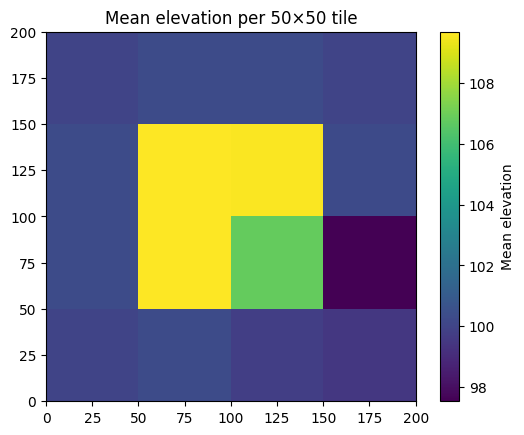
Spatial Statistics by Region

Combining statistics(inside_polygon=...) with systematic spatial partitioning yields a spatial analysis.

from shapely.geometry import box

# Divide the domain into a 4×4 grid and compute mean elevation per tile
tile_size = 50
means = np.zeros((4, 4))
for i in range(4):
    for j in range(4):
        poly = box(i * tile_size, j * tile_size,
                   (i + 1) * tile_size, (j + 1) * tile_size)
        s = dem.statistics(inside_polygon=poly)
        means[i, j] = s['Mean']

fig, ax = plt.subplots()
im = ax.imshow(means.T, origin='lower', extent=[0, 200, 0, 200])
plt.colorbar(im, ax=ax, label='Mean elevation')
ax.set_title('Mean elevation per 50×50 tile')

Text(0.5, 1.0, 'Mean elevation per 50×50 tile')

Cropping and Edge Trimming

• crop_array(bbox) — extract a subregion by world coordinates

• crop_masked_at_edges() — automatically trim rows/columns that are fully masked at the edges

# Mask outside a circle, then trim
circle_dem = WolfArray(mold=dem)
dist = np.sqrt((X - 0.)**2 + (Y - 0.)**2)
circle_dem.array[dist > 2.] = circle_dem.nullvalue
circle_dem.mask_data(circle_dem.nullvalue)

trimmed = circle_dem.crop_masked_at_edges()
print(f"Before trim: {circle_dem.array.shape}")
print(f"After  trim: {trimmed.array.shape}")
trimmed.plot_matplotlib()

Before trim: (200, 200)
After  trim: (132, 132)

(<Figure size 640x480 with 1 Axes>, <Axes: >)