Hydraulic utilities

This tutorial covers two utility modules:

1. ``compare_series`` — model evaluation metrics (NSE, KGE, RMSE, …)

2. ``friction_law`` — pipe/channel friction coefficients (Colebrook, Barr-Bathurst)

Part 1 — compare_series: model evaluation metrics

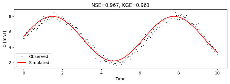
Compare observed vs. simulated time series using standard hydrological metrics.

import numpy as np
from wolfhece.compare_series import (
    Nash_Sutcliffe_efficiency,
    Kling_Gupta_efficiency,
    Root_Mean_Square_Error,
    Mean_Absolute_Error,
    Pearson_Correlation_Coefficient,
)

# Synthetic example: observed vs. simulated discharge
np.random.seed(42)
t = np.linspace(0, 10, 200)
observed  = 5.0 + 3.0 * np.sin(t) + np.random.normal(0, 0.3, len(t))
simulated = 5.1 + 2.9 * np.sin(t + 0.1)

nse  = Nash_Sutcliffe_efficiency(observed, simulated)
kge  = Kling_Gupta_efficiency(observed, simulated)
rmse = Root_Mean_Square_Error(observed, simulated)
mae  = Mean_Absolute_Error(observed, simulated)
r    = Pearson_Correlation_Coefficient(observed, simulated)

print(f"NSE  = {nse:.4f}  (1 = perfect)")
print(f"KGE  = {kge:.4f}  (1 = perfect)")
print(f"RMSE = {rmse:.4f}")
print(f"MAE  = {mae:.4f}")
print(f"r    = {r:.4f}")

NSE  = 0.9671  (1 = perfect)
KGE  = 0.9609  (1 = perfect)
RMSE = 0.3644
MAE  = 0.2981
r    = 0.9843

import matplotlib.pyplot as plt

fig, ax = plt.subplots(figsize=(8, 3))
ax.plot(t, observed, 'k.', ms=2, label='Observed')
ax.plot(t, simulated, 'r-', label='Simulated')
ax.set_xlabel('Time'); ax.set_ylabel('Q [m³/s]')
ax.set_title(f'NSE={nse:.3f}, KGE={kge:.3f}')
ax.legend()
plt.tight_layout(); plt.show()

Available metrics

Function	Metric
Nash_Sutcliffe_efficiency	NSE
Kling_Gupta_efficiency	KGE
modified_Kling_Gupta_efficiency	KGE’ (CV-based)
Root_Mean_Square_Error	RMSE
Mean_Absolute_Error	MAE
Mean_Absolute_Percentage_Error	MAPE
Pearson_Correlation_Coefficient	Pearson r
Spearman_Rank_Correlation_Coefficient	Spearman ρ
Dynamic_Time_Warping_distance	DTW distance
normalize_series	Normalize to [0,1]

---

Part 2 — friction_law: hydraulic friction coefficients

Numba-accelerated friction factor computations for pipe/channel flows.

from wolfhece.friction_law import f_colebrook, f_barr_bathurst

# Friction factor for a smooth pipe
k_sur_D = 0.001   # relative roughness k/D
Re = 1e5           # Reynolds number

f_cole = f_colebrook(k_sur_D, Re)
f_barr = f_barr_bathurst(k_sur_D, Re)

print(f"Colebrook      : f = {f_cole:.6f}")
print(f"Barr-Bathurst  : f = {f_barr:.6f}")

Colebrook      : f = 0.022175
Barr-Bathurst  : f = 0.022184

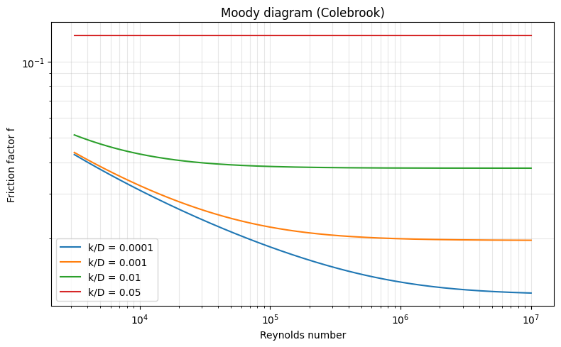
# Moody diagram: f vs. Re for various roughness values
Re_values = np.logspace(3.5, 7, 200)
roughness = [0.0001, 0.001, 0.01, 0.05]

fig, ax = plt.subplots(figsize=(8, 5))
for k_D in roughness:
    f_vals = [f_colebrook(k_D, Re) for Re in Re_values]
    ax.loglog(Re_values, f_vals, label=f'k/D = {k_D}')

ax.set_xlabel('Reynolds number')
ax.set_ylabel('Friction factor f')
ax.set_title('Moody diagram (Colebrook)')
ax.legend()
ax.grid(True, which='both', alpha=0.3)
plt.tight_layout(); plt.show()

Available functions

Function	Description
f_colebrook(k/D, Re)	Colebrook with laminar/turbulent transitions
f_colebrook_pure(k/D, Re)	Pure iterative Colebrook (turbulent only)
f_barr_bathurst(k/D, Re)	Barr-Bathurst approximation

Note: For open-channel flow, use \(Re' = 4 \cdot Re\) (hydraulic radius convention).