Cross-Sections

The crosssections module provides tools for managing river cross-section profiles.

A ``profile`` extends vector and represents a single cross-section with:

• 3D coordinates where X = curvilinear abscissa and Z = elevation

• Reference points: left bank, right bank, bed

• Hydraulic property calculations (wet area, wetted perimeter, hydraulic radius)

The ``crosssections`` class manages a collection of profiles loaded from various formats:

• '2022' — Wolf text format

• '2025_xlsx' — Excel spreadsheet

• 'vecz' — Wolf vector with Z

• 'sxy' — SPW/SETHY format

This tutorial demonstrates creating and manipulating cross-sections programmatically.

import numpy as np
import matplotlib.pyplot as plt
from wolfhece.PyCrosssections import profile, crosssections, postype

Creating a Profile from Scratch

A profile stores survey data as (curvilinear abscissa, 0, elevation) vertices.

# Trapezoidal channel cross-section
s = np.array([0, 2, 4, 8, 12, 14, 16])     # curvilinear abscissa [m]
z = np.array([5, 5, 2, 1, 2, 5, 5])         # elevation [m]

# Build the (s, z) array – profile expects 2 columns
coords = np.column_stack([s, z])

p = profile(name='CS1', data_sect=coords)
print(f"Profile '{p.myname}': {p.nbvertices} vertices")
print(f"S range: {s[0]:.1f} – {s[-1]:.1f} m")

Profile 'CS1': 7 vertices
S range: 0.0 – 16.0 m

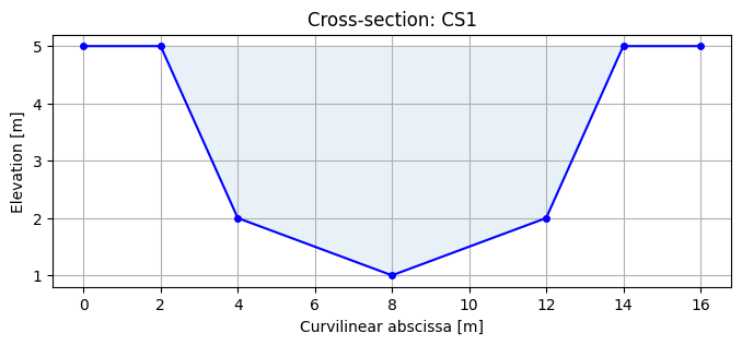
Plotting a Profile

fig, ax = plt.subplots(figsize=(8, 3))
ax.plot(s, z, 'b-o', markersize=4)
ax.fill_between(s, z, z.max(), alpha=0.1)
ax.set_xlabel('Curvilinear abscissa [m]')
ax.set_ylabel('Elevation [m]')
ax.set_title(f'Cross-section: {p.myname}')
ax.grid(True)

Reference Points

A profile can store reference positions for the left bank, right bank, and bed. These are used for hydraulic calculations and for aligning profiles along a river.

# Set reference points using vertex indices
# Vertices: s=[0,2,4,8,12,14,16]  z=[5,5,2,1,2,5,5]
# Index:      0 1 2 3  4   5  6
p.banksbed_postype = postype.BY_INDEX
p.bankleft = 2    # vertex at s=4m
p.bankright = 4   # vertex at s=12m
p.bed = 3         # vertex at s=8m, z=1m

bl = p.bankleft_vertex
br = p.bankright_vertex
bd = p.bed_vertex
print(f"Left bank at s={bl.x}, z={bl.z}")
print(f"Right bank at s={br.x}, z={br.z}")
print(f"Bed at s={bd.x}, z={bd.z}")

Left bank at s=4.0, z=2.0
Right bank at s=12.0, z=2.0
Bed at s=8.0, z=1.0

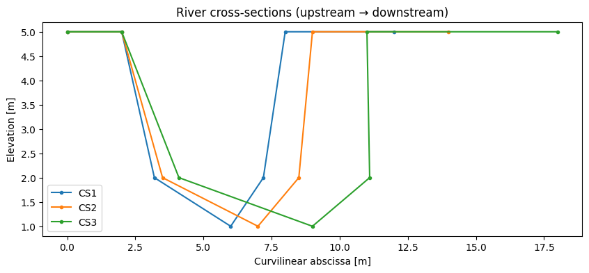
Working with Multiple Cross-Sections

In practice, cross-sections are loaded from files via crosssections(filename, format=...).

Here we demonstrate creating a simple collection programmatically.

# Create three profiles with gradually widening channel
profiles = []
for i, width in enumerate([8, 10, 14]):
    half = width / 2
    s_i = np.array([0, 2, 2+half*0.3, 2+half, 2+half+half*0.3, 2+half+2, 4+width])
    z_i = np.array([5, 5, 2, 1, 2, 5, 5])
    coords_i = np.column_stack([s_i, z_i])  # 2 columns: (s, z)
    p_i = profile(name=f'CS{i+1}', data_sect=coords_i)
    profiles.append(p_i)

fig, ax = plt.subplots(figsize=(10, 4))
for p_i in profiles:
    xs = [v.x for v in p_i.myvertices]
    zs = [v.z for v in p_i.myvertices]
    ax.plot(xs, zs, '-o', markersize=3, label=p_i.myname)

ax.set_xlabel('Curvilinear abscissa [m]')
ax.set_ylabel('Elevation [m]')
ax.set_title('River cross-sections (upstream → downstream)')
ax.legend()
plt.show()

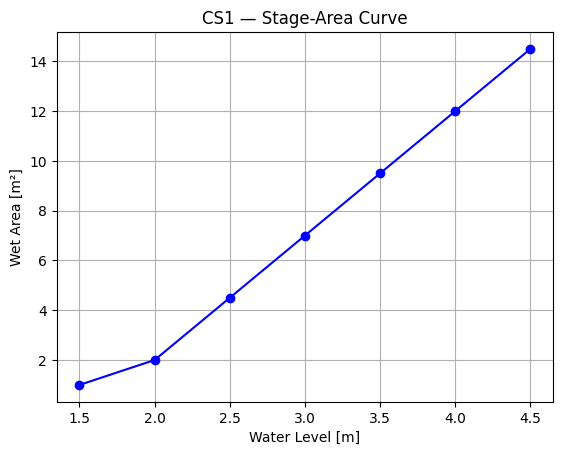
Hydraulic Calculations

A profile can compute basic hydraulic properties for a given water level:

• Wet area

• Wetted perimeter

• Hydraulic radius

These are computed from the cross-section geometry with the wetarea, wetperimeter, and hydraulicradius attributes after setting the water surface level.

# Compute wet properties for the first profile at different water levels
p1 = profiles[0]
xs_p1 = np.array([v.x for v in p1.myvertices])
zs_p1 = np.array([v.z for v in p1.myvertices])

water_levels = np.linspace(1.5, 4.5, 7)
areas = []
for wl in water_levels:
    # Compute wet area by trapezoidal integration under water level
    clipped_z = np.minimum(zs_p1, wl)
    area = np.trapezoid(wl - clipped_z, xs_p1)
    areas.append(area)

fig, ax = plt.subplots()
ax.plot(water_levels, areas, '-o', color='blue')
ax.set_xlabel('Water Level [m]')
ax.set_ylabel('Wet Area [m²]')
ax.set_title(f'{p1.myname} — Stage-Area Curve')
ax.grid(True)
plt.show()

Loading Cross-Sections from Files

In real applications, cross-sections are loaded from survey data files:

# Wolf 2022 text format
cs = crosssections('path/to/sections.txt', format='2022')

# Excel format (requires openpyxl)
cs = crosssections('path/to/sections.xlsx', format='2025_xlsx')

# Wolf vector format with Z
cs = crosssections('path/to/sections.vecz', format='vecz')

# SPW/SETHY format
cs = crosssections('path/to/sections.sxy', format='sxy')

After loading, profiles are available in cs.myprofiles, a dict keyed by 'cs', 'index', 'left', 'bed', 'right'.