WolfArray — File I/O

Note — All I/O operations shown here work identically on WolfArrayModel (no GUI dependency). See the Model/GUI architecture tutorial for details.

A WolfArray supports multiple file formats. The constructor auto-detects the format from the file extension:

Extension	Format	CRS embedded?
.bin	Wolf binary (default)	No (separate .prj sidecar)
.tif / .tiff	GeoTIFF	Yes
.vrt	GDAL Virtual Raster	Yes
.npy	NumPy binary	No
.flt	Binary raster	No

The Wolf binary format stores an auxiliary header file alongside the data file.

from wolfhece.wolf_array import WolfArray, header_wolf
import numpy as np
import tempfile, os, shutil

Creating a Sample Array

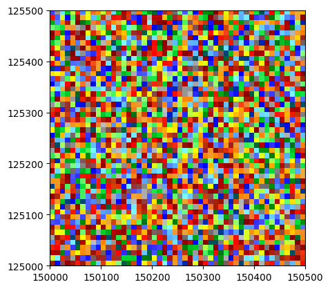
We first build a small array to use throughout this tutorial.

h = header_wolf()
h.shape = (50, 50)
h.set_resolution(10., 10.)   # 10 m per pixel
h.set_origin(150000., 125000.)  # Belgian Lambert 72

wa = WolfArray(srcheader=h)
rng = np.random.default_rng(42)
wa.array[:, :] = rng.uniform(50., 200., size=(50, 50))
wa.plot_matplotlib()

(<Figure size 640x480 with 1 Axes>, <Axes: >)

Saving as Wolf Binary (.bin)

The .bin format is the native WOLF format. write_all() creates the binary data file and a companion header file.

tmpdir = tempfile.mkdtemp()

bin_path = os.path.join(tmpdir, 'demo.bin')
wa.write_all(bin_path)
print('Files created:', sorted(os.listdir(tmpdir)))

Files created: ['demo.bin', 'demo.bin.txt']

# Reload from Wolf binary
wa_bin = WolfArray(fname=bin_path)
print(wa_bin)
print('Data match:', np.allclose(wa.array.data, wa_bin.array.data))

Shape  : 50 x 50
Resolution  : 10.0 x 10.0
Spatial extent :
   - Origin : (150000.0 ; 125000.0)
   - End : (150500.0 ; 125500.0)
   - Width x Height : 500.0 x 500.0
   - Translation : (0.0 ; 0.0)
Null value : 0.0


Data match: True

Saving as GeoTIFF (.tif)

GeoTIFF embeds georeferencing and coordinate reference system. Use the EPSG parameter to specify the CRS.

EPSG 31370 = Belgian Lambert 72 (the default in Wolf).

tif_path = os.path.join(tmpdir, 'demo.tif')
wa.write_all(tif_path, EPSG=31370)
print('GeoTIFF created:', os.path.exists(tif_path))

GeoTIFF created: True

# Reload from GeoTIFF
wa_tif = WolfArray(fname=tif_path)
print(wa_tif)
print('Data match:', np.allclose(wa.array.data, wa_tif.array.data))

Shape  : 50 x 50
Resolution  : 10.0 x 10.0
Spatial extent :
   - Origin : (150000.0 ; 125000.0)
   - End : (150500.0 ; 125500.0)
   - Width x Height : 500.0 x 500.0
   - Translation : (0.0 ; 0.0)
Null value : 0.0


Data match: True

Saving as NumPy (.npy)

The .npy format stores only the raw array data — no georeferencing.

npy_path = os.path.join(tmpdir, 'demo.npy')
wa.write_all(npy_path)
print('NumPy file created:', os.path.exists(npy_path))

# Raw NumPy load (no header)
raw = np.load(npy_path)
print('Shape:', raw.shape)

NumPy file created: True
Shape: (50, 50)

Importing GeoTIFF with import_geotif

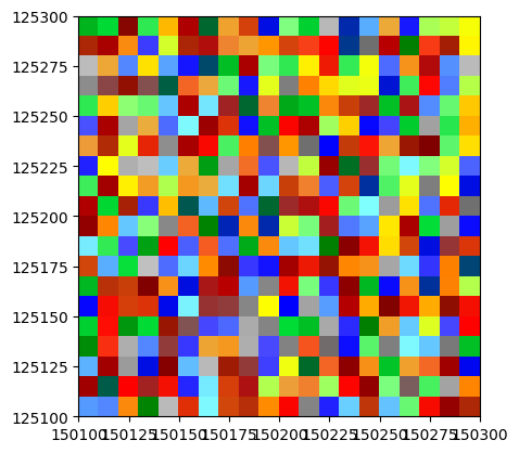
The import_geotif() method offers extra options:

• which — band index (1-based) for multi-band rasters

• crop — bounding box [xmin, xmax, ymin, ymax] to read only a subregion

# Reload with spatial crop — crop format is [xmin, xmax, ymin, ymax]
wa_crop = WolfArray()
wa_crop.import_geotif(tif_path, crop=[150100., 150300., 125100., 125300.])
print(wa_crop)
wa_crop.plot_matplotlib()

Shape  : 20 x 20
Resolution  : 10.0 x 10.0
Spatial extent :
   - Origin : (150100.0 ; 125100.0)
   - End : (150300.0 ; 125300.0)
   - Width x Height : 200.0 x 200.0
   - Translation : (0.0 ; 0.0)
Null value : 0.0

(<Figure size 640x480 with 1 Axes>, <Axes: >)

Exporting with export_geotif

export_geotif() gives fine control over the output directory, extent, and EPSG code.

outdir = os.path.join(tmpdir, 'geotif_export')
os.makedirs(outdir, exist_ok=True)
wa.export_geotif(outdir=outdir, EPSG=31370)
print('Exported files:', os.listdir(outdir))

Exported files: ['.tif']

Clean Up

shutil.rmtree(tmpdir, ignore_errors=True)
print('Temporary files removed.')

Temporary files removed.