Raster–Vector Operations

Note — All operations shown here work identically on WolfArrayModel / vectorModel / zoneModel (no GUI dependency). See the Model/GUI architecture tutorial for details.

WolfArray provides a rich set of methods that combine raster data with vector geometries (polygons, polylines):

• Masking cells inside / outside polygons

• Extracting values inside a polygon or under a polyline

• Interpolating Z-values from vector vertices onto the raster grid

• Cropping to a bounding box

from wolfhece.wolf_array import WolfArray, header_wolf
from wolfhece.PyVertexvectors import vector, zone, wolfvertex
import numpy as np
import matplotlib.pyplot as plt

Setup: a DEM-like Raster and a Polygon

h = header_wolf()
h.shape = (100, 100)
h.set_resolution(1., 1.)
h.set_origin(0., 0.)

dem = WolfArray(srcheader=h)
# Synthetic terrain: a saddle surface
x = np.linspace(-1, 1, 100)
y = np.linspace(-1, 1, 100)
X, Y = np.meshgrid(x, y, indexing='ij')  # F-order indexing
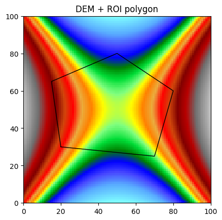
dem.array[:, :] = 100. + 20. * X**2 - 15. * Y**2

# A polygon defining a region of interest
roi = vector(name='ROI')
roi.add_vertices_from_array(np.array([
    [20, 30], [70, 25], [80, 60], [50, 80], [15, 65]
]))
roi.closed = True
roi.find_minmax()

fig, ax = dem.plot_matplotlib()
roi.plot_matplotlib(ax)
ax.set_title('DEM + ROI polygon')

Text(0.5, 1.0, 'DEM + ROI polygon')

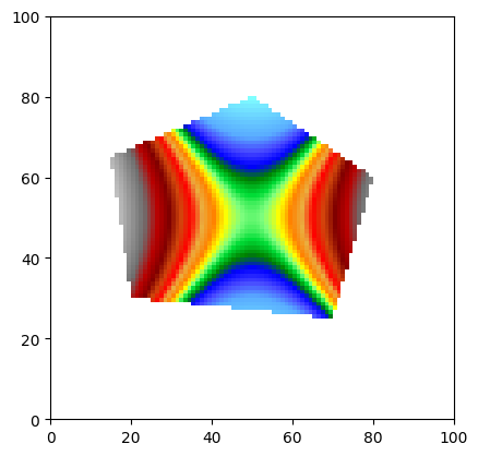
Masking Outside a Polygon

mask_outsidepoly() masks all cells whose center falls outside the given polygon. This is the typical “clip to boundary” operation.

clipped = WolfArray(mold=dem)  # copy
clipped.mask_outsidepoly(roi)
clipped.plot_matplotlib()
print(f"Valid cells after clip: {clipped.count()} / {dem.count()}")

Valid cells after clip: 2595 / 10000

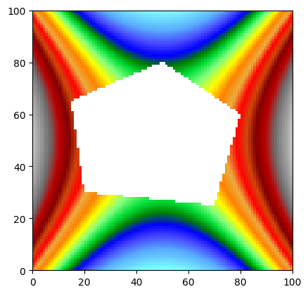
Masking Inside a Polygon

mask_insidepoly() does the opposite — it removes cells inside the polygon.

hole = WolfArray(mold=dem)
hole.mask_insidepoly(roi)
hole.plot_matplotlib()
print(f"Valid cells with hole: {hole.count()}")

Valid cells with hole: 7395

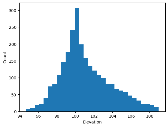
Extracting Values Inside a Polygon

get_values_insidepoly() returns the array values (and optionally their coordinates) that fall inside the polygon.

vals, xy = dem.get_values_insidepoly(roi, getxy=True)
print(f"Number of cells inside polygon: {len(vals)}")
print(f"Elevation range: {vals.min():.2f} – {vals.max():.2f}")

# Show histogram
fig, ax = plt.subplots()
ax.hist(vals, bins=30)
ax.set_xlabel('Elevation')
ax.set_ylabel('Count')

Number of cells inside polygon: 2595
Elevation range: 94.67 – 108.98

Text(0, 0.5, 'Count')

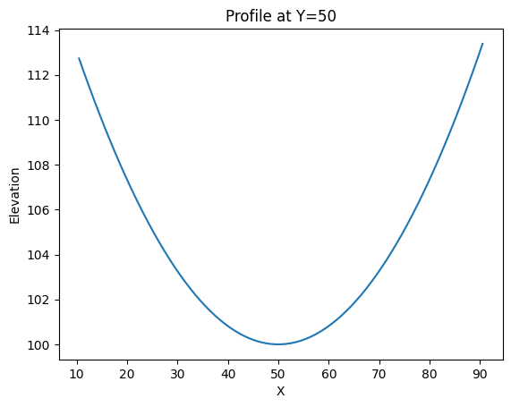
Extracting Values along a Polyline

get_values_underpoly() returns values along a polyline (profile extraction).

profile_line = vector(name='profile')
profile_line.add_vertices_from_array(np.array([[10, 50], [90, 50]]))
profile_line.find_minmax()

vals_under = dem.get_values_underpoly(profile_line, getxy=True)
print(f"Cells under profile: {len(vals_under[0])}")

xy = np.array(vals_under[1])  # convert list to numpy array

fig, ax = plt.subplots()
ax.plot(xy[:, 0], vals_under[0])  # x-coordinate vs elevation
ax.set_xlabel('X')
ax.set_ylabel('Elevation')
ax.set_title('Profile at Y=50')
plt.show()

Cells under profile: 81

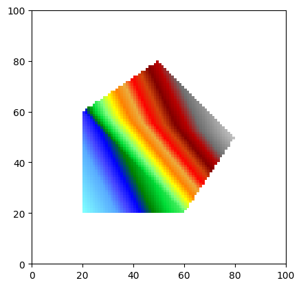
Interpolating on a Polygon

interpolate_on_polygon() fills raster cells inside a polygon by interpolating from vertex Z-values using SciPy griddata (linear, nearest, or cubic).

# Create a polygon with Z-values at vertices
interp_poly = vector(name='interp_region')
interp_poly.add_vertices_from_array(np.array([
    [20, 20, 80],
    [60, 20, 90],
    [80, 50, 120],
    [50, 80, 110],
    [20, 60, 85]
]))
interp_poly.closed = True
interp_poly.find_minmax()

flat = WolfArray(srcheader=h)
flat.array[:, :] = 0.
flat.nullvalue = 0.
flat.interpolate_on_polygon(interp_poly, method='linear')
flat.plot_matplotlib()

(<Figure size 640x480 with 1 Axes>, <Axes: >)

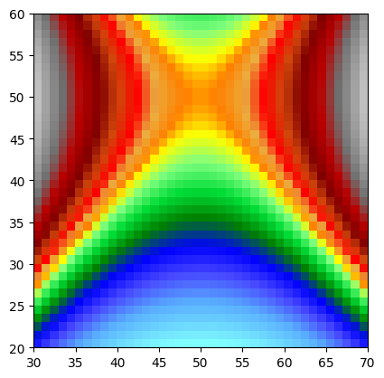
Cropping to a Bounding Box

crop_array() returns a new WolfArray trimmed to the given bounding box [[xmin, xmax], [ymin, ymax]].

cropped = dem.crop_array([[30, 70], [20, 60]])
print(cropped)
cropped.plot_matplotlib()

Shape  : 40 x 40
Resolution  : 1.0 x 1.0
Spatial extent :
   - Origin : (30.0 ; 20.0)
   - End : (70.0 ; 60.0)
   - Width x Height : 40.0 x 40.0
   - Translation : (0.0 ; 0.0)
Null value : 0.0

(<Figure size 640x480 with 1 Axes>, <Axes: >)

Zonal Statistics

Combine statistics(inside_polygon=...) with a list of polygons for zonal statistics.

from shapely.geometry import box

zones_list = [
    ('NW', box(5, 55, 45, 95)),
    ('NE', box(55, 55, 95, 95)),
    ('SW', box(5, 5, 45, 45)),
    ('SE', box(55, 5, 95, 45)),
]

for name, poly in zones_list:
    s = dem.statistics(inside_polygon=poly)
    print(f"{name}: mean={s['Mean']:.2f}, std={s['Std']:.2f}, "
          f"min={s['Min']:.2f}, max={s['Max']:.2f}")

NW: mean=101.55, std=6.01, min=88.12, max=115.98
NE: mean=101.55, std=6.01, min=88.12, max=115.98
SW: mean=101.55, std=6.01, min=88.12, max=115.98
SE: mean=101.55, std=6.01, min=88.12, max=115.98