Multi-Criteria Analysis — Usage Example

This notebook demonstrates how to use the MulticriteriAnalysis class from wolfhece.multicriteria.analysis.

Core concept

The analysis works in two stages:

1. Binary scoring — Each input array is evaluated cell-by-cell against a condition (e.g. ≥ threshold). Every cell receives a binary score: 1 (condition met) or 0 (condition not met).

2. Score combination — The binary scores from all inputs are combined using a chosen method: sum, average, or percentage.

Input array 1  ──► [condition + threshold] ──► binary score 1 ─┐
Input array 2  ──► [condition + threshold] ──► binary score 2 ─┼──► combined result
Input array 3  ──► [condition + threshold] ──► binary score 3 ─┘

1. Imports

import numpy as np
import matplotlib.pyplot as plt
import matplotlib.colors as mcolors

from wolfhece.multicriteria.analysis import (
    Input,
    MulticriteriAnalysis,
    Operator,
)

2. Create three synthetic input arrays

We simulate three spatially distributed variables on a 6×6 grid:

Variable	Physical meaning	Condition	Threshold
water_depth	Water depth (m)	≥	0.3 m
velocity	Flow velocity (m/s)	≥	0.5 m/s
hazard_index	Hazard index (–)	≥	2.0

A cell is “dangerous” (score = 1) when its value meets the condition.

# Reproducibility
rng = np.random.default_rng(seed=42)

shape = (6, 6)

# --- Water depth (m) ---
water_depth = np.ma.MaskedArray(data=rng.uniform(0.0, 1.0, shape).astype(np.float32), mask=False)

# --- Flow velocity (m/s) ---
velocity = np.ma.MaskedArray(data=rng.uniform(0.0, 1.5, shape).astype(np.float32), mask=False)

# --- Hazard index (dimensionless) ---
hazard_index = np.ma.MaskedArray(data=rng.uniform(0.0, 4.0, shape).astype(np.float32), mask=False)

print("water_depth:\n", np.round(water_depth, 2))
print("\nvelocity:\n", np.round(velocity, 2))
print("\nhazard_index:\n", np.round(hazard_index, 2))

water_depth:
 [[0.7699999809265137 0.4399999976158142 0.8600000143051147
  0.699999988079071 0.09000000357627869 0.9800000190734863]
 [0.7599999904632568 0.7900000214576721 0.12999999523162842
  0.44999998807907104 0.3700000047683716 0.9300000071525574]
 [0.6399999856948853 0.8199999928474426 0.4399999976158142
  0.23000000417232513 0.550000011920929 0.05999999865889549]
 [0.8299999833106995 0.6299999952316284 0.7599999904632568
  0.3499999940395355 0.9700000286102295 0.8899999856948853]
 [0.7799999713897705 0.1899999976158142 0.4699999988079071
  0.03999999910593033 0.15000000596046448 0.6800000071525574]
 [0.7400000095367432 0.9700000286102295 0.33000001311302185
  0.3700000047683716 0.4699999988079071 0.1899999976158142]]

velocity:
 [[0.1899999976158142 0.7099999785423279 0.3400000035762787 1.0
  0.6600000262260437 1.25]
 [1.0499999523162842 0.4699999988079071 1.25 1.2100000381469727
  0.5799999833106995 0.4300000071525574]
 [1.0199999809265137 0.20999999344348907 0.30000001192092896
  0.009999999776482582 1.1799999475479126 1.0]
 [1.059999942779541 1.1699999570846558 0.6899999976158142
  0.8500000238418579 0.20999999344348907 0.17000000178813934]
 [1.0 0.7099999785423279 0.8500000238418579 1.149999976158142
  0.949999988079071 0.8299999833106995]
 [0.8399999737739563 0.46000000834465027 0.05000000074505806
  0.6600000262260437 0.3199999928474426 0.6100000143051147]]

hazard_index:
 [[3.4100000858306885 0.9399999976158142 0.23000000417232513
  1.1299999952316284 1.1699999570846558 2.6500000953674316]
 [2.2300000190734863 3.140000104904175 2.6600000858306885
  1.6299999952316284 3.259999990463257 0.6700000166893005]
 [0.09000000357627869 0.36000001430511475 2.890000104904175
  1.850000023841858 0.6499999761581421 2.0]
 [0.6100000143051147 2.7899999618530273 1.7799999713897705
  1.5199999809265137 1.2100000381469727 2.5199999809265137]
 [1.4500000476837158 0.3499999940395355 0.4699999988079071
  3.8499999046325684 3.630000114440918 2.799999952316284]
 [1.059999942779541 3.880000114440918 3.119999885559082 2.869999885559082
  1.7999999523162842 1.090000033378601]]

3. Wrap each array in an Input object

An Input bundles together:

• the data array,

• the condition used to score it (Operator.*),

• the threshold value.

input_depth = Input(name="water_depth",
                    array=water_depth,
                    condition=Operator.SUPERIOR_OR_EQUAL,
                    threshold=0.3)

input_velocity = Input(name="velocity",
                       array=velocity,
                       condition=Operator.SUPERIOR_OR_EQUAL,
                       threshold=0.5)

input_hazard = Input(name="hazard_index",
                     array=hazard_index,
                     condition=Operator.SUPERIOR_OR_EQUAL,
                     threshold=2.0)

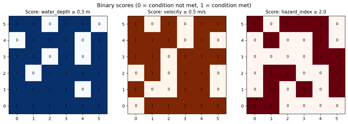
4. Visualise the binary scores

Before combining, inspect the individual binary score of each input. A cell is white (0 — condition not met) or coloured (1 — condition met).

def plot_binary(ax, data, title, threshold, cmap="Blues"):
    im = ax.imshow(data.T, origin="lower", cmap=cmap, vmin=0, vmax=1)
    ax.set_title(title, fontsize=11)
    for i in range(data.shape[0]):
        for j in range(data.shape[1]):
            ax.text(i, j, str(int(data[i, j])), ha="center", va="center", fontsize=9)
    return im

fig, axes = plt.subplots(1, 3, figsize=(12, 4))

score_depth   = input_depth.score.score
score_vel     = input_velocity.score.score
score_hazard  = input_hazard.score.score

plot_binary(axes[0], score_depth,  "Score: water_depth ≥ 0.3 m",   0.3, cmap="Blues")
plot_binary(axes[1], score_vel,    "Score: velocity ≥ 0.5 m/s",    0.5, cmap="Oranges")
plot_binary(axes[2], score_hazard, "Score: hazard_index ≥ 2.0",    2.0, cmap="Reds")

fig.suptitle("Binary scores (0 = condition not met, 1 = condition met)", fontsize=13)
plt.tight_layout()
plt.show()

5. Run the MulticriteriAnalysis

Three combination methods are available:

Method	Formula	Range
SUM	\(\sum_i s_i\)	\([0, N]\)
AVERAGE	\(\frac{1}{N}\sum_i s_i\)	\([0, 1]\)
PERCENTAGE	\(\frac{100}{N}\sum_i s_i\)	\([0, 100]\)

where \(N\) is the number of inputs and \(s_i \in \{0,1\}\).

inputs = [input_depth, input_velocity, input_hazard]

mca_sum = MulticriteriAnalysis(inputs=inputs, method=Operator.SUM)
mca_avg = MulticriteriAnalysis(inputs=inputs, method=Operator.AVERAGE)
mca_pct = MulticriteriAnalysis(inputs=inputs, method=Operator.PERCENTAGE)

result_sum = mca_sum.results.array
result_avg = mca_avg.results.array
result_pct = mca_pct.results.array

print("SUM result (integer, range [0, 3]):\n",    result_sum)
print("\nAVERAGE result (float, range [0, 1]):\n", np.round(result_avg, 2))
print("\nPERCENTAGE result (%, range [0, 100]):\n", np.round(result_pct, 1))

WARNING:root:No weight provided. Setting weight to equal distribution.
WARNING:root:No weight provided. Setting weight to equal distribution.
WARNING:root:No weight provided. Setting weight to equal distribution.
WARNING:root:No weight provided. Setting weight to equal distribution.
WARNING:root:No weight provided. Setting weight to equal distribution.
WARNING:root:No weight provided. Setting weight to equal distribution.

SUM result (integer, range [0, 3]):
 [[2 2 1 2 1 3]
 [3 2 2 2 3 1]
 [2 1 2 0 2 2]
 [2 3 2 2 1 2]
 [2 1 2 2 2 3]
 [2 2 2 3 1 1]]

AVERAGE result (float, range [0, 1]):
 [[0.6700000166893005 0.6700000166893005 0.33000001311302185
  0.6700000166893005 0.33000001311302185 1.0]
 [1.0 0.6700000166893005 0.6700000166893005 0.6700000166893005 1.0
  0.33000001311302185]
 [0.6700000166893005 0.33000001311302185 0.6700000166893005 0.0
  0.6700000166893005 0.6700000166893005]
 [0.6700000166893005 1.0 0.6700000166893005 0.6700000166893005
  0.33000001311302185 0.6700000166893005]
 [0.6700000166893005 0.33000001311302185 0.6700000166893005
  0.6700000166893005 0.6700000166893005 1.0]
 [0.6700000166893005 0.6700000166893005 0.6700000166893005 1.0
  0.33000001311302185 0.33000001311302185]]

PERCENTAGE result (%, range [0, 100]):
 [[66.7 66.7 33.3 66.7 33.3 100.0]
 [100.0 66.7 66.7 66.7 100.0 33.3]
 [66.7 33.3 66.7 0.0 66.7 66.7]
 [66.7 100.0 66.7 66.7 33.3 66.7]
 [66.7 33.3 66.7 66.7 66.7 100.0]
 [66.7 66.7 66.7 100.0 33.3 33.3]]

6. Visualise the combined results

fig, axes = plt.subplots(1, 3, figsize=(14, 4))

def plot_result(ax, data, title, vmin, vmax, fmt="{:.0f}", cmap="YlOrRd"):
    im = ax.imshow(data.T, origin="lower", cmap=cmap, vmin=vmin, vmax=vmax)
    ax.set_title(title, fontsize=11)
    plt.colorbar(im, ax=ax, shrink=0.75)
    for i in range(data.shape[0]):
        for j in range(data.shape[1]):
            ax.text(i, j, fmt.format(data[i, j]), ha="center", va="center", fontsize=8)

plot_result(axes[0], result_sum, "SUM  [0 – 3]",   vmin=0, vmax=3,   fmt="{:.0f}")
plot_result(axes[1], result_avg, "AVERAGE  [0 – 1]", vmin=0, vmax=1, fmt="{:.2f}")
plot_result(axes[2], result_pct, "PERCENTAGE  [0 – 100 %]", vmin=0, vmax=100, fmt="{:.0f}")

fig.suptitle(
    "Combined multi-criteria results\n"
    "(higher value = more criteria simultaneously satisfied)",
    fontsize=13,
)
plt.tight_layout()
plt.show()

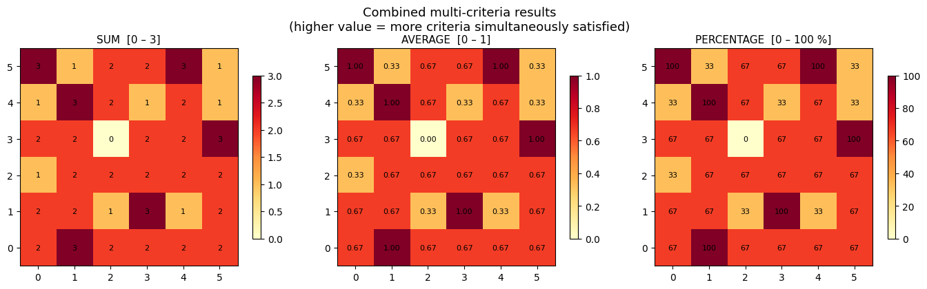
7. Key takeaways

• Each input is scored independently and binaryly: 1 if the condition is met, 0 otherwise.

• The final result reflects how many criteria are simultaneously satisfied at each spatial location.

• The PERCENTAGE method is the most intuitive: 100 % means all criteria are met, 0 % means none.

• Any Operator condition can be used per input (SUPERIOR, INFERIOR, BETWEEN, OUTSIDE, etc.).

• A mold (WolfArray) can be supplied to transfer geo-spatial metadata (origin, resolution, CRS) onto the result.

• ‘results’ is a WolfArray object, so it can be easily added to a Wolf viewer