Analyse d’une matrice sur base de polygones et projection sur une trace

Import des modules

try:
    from wolfhece import is_enough
    if not is_enough('2.2.63'):
        raise ImportError("Please update wolfhece to at least version 2.2.31")
except ImportError:
    raise ImportError("Please install the required version of wolfhece: pip install wolfhece>=2.2.30")

from wolfhece.analyze_poly import Array_analysis_polygons, Array_analysis_onepolygon
from wolfhece.wolf_array import WolfArray, header_wolf
from wolfhece.PyVertexvectors import vector, zone, Zones, wolfvertex as wv

import matplotlib.pyplot as plt
import numpy as np

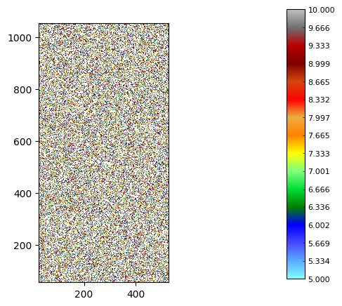
Création d’une matrice de variables aléatoires

h = header_wolf()
h.set_origin(25, 55) # Set the origin (lower-left) of the array
h.set_resolution(0.5 , 0.5) # Set the resolution of the array
h.shape = (1000, 2000) # Set the shape of the array (cells along x and y axes)

a = WolfArray(srcheader= h)

a.array[:,:] = np.random.rand(1000, 2000) * 10
a.mask_lower(5.)
a.set_nullvalue_in_mask()

a.plot_matplotlib(with_legend= True)
print("Number of values in the array:", a.nbnotnull)

Number of values in the array: 1000080

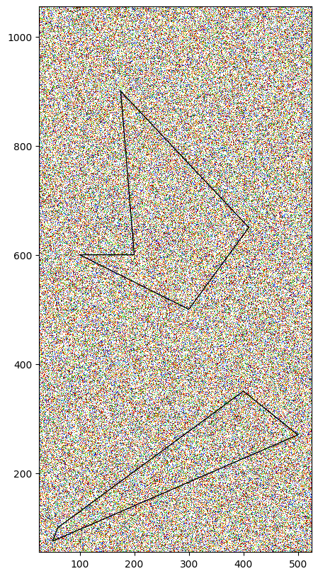
Création de polygones d’analyse

Pour l’exemple, on va définir deux polygones.

# Create polygons
zone_poly = zone(name = 'polygons')

poly1 = vector(name=f'Polygon_1', parentzone=zone_poly)
poly1.add_vertices_from_array(np.array([[60, 100],
                                        [400, 350],
                                        [500, 270],
                                        [50, 75]]))
poly1.force_to_close()  # Ensure the polygon is closed

poly2 = vector(name=f'Polygon_2', parentzone=zone_poly)
poly2.add_vertices_from_array(np.array([[410, 650],
                                        [175, 900],
                                        [200, 600],
                                        [100, 600],
                                        [300, 500]]))
poly2.force_to_close()  # Ensure the polygon is closed

zone_poly.add_vector(poly1)
zone_poly.add_vector(poly2)

fig, ax = plt.subplots(figsize=(10, 10))
a.plot_matplotlib(figax = (fig, ax))
zone_poly.plot_matplotlib(ax)
ax.set_aspect('equal')

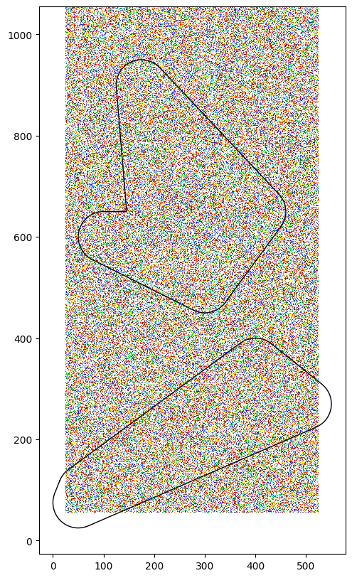
Création de l’objet d’analyse avec buffer

Il est possible de définir un buffer autour des polygones. Le buffer est une zone supplémentaire qui permet d’inclure des valeurs adjacentes aux polygones dans l’analyse.

Si un buffer est défini, le polygone sera une copie du polygone original avec un buffer de la taille définie. Autrement, le polygone est un pointeur vers le polygone original.

analyze = Array_analysis_polygons(a, zone_poly, buffer_size= 50.)

fig, ax = plt.subplots(figsize=(10, 10))
a.plot_matplotlib(figax = (fig, ax))
analyze.polygons.plot_matplotlib(ax)
ax.set_aspect('equal')

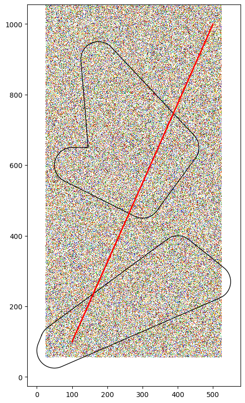
Création d’une polyligne sur laquelle projeter

Le but est d’obtenir les valeurs du polygone dont son centroïde est projeté sur la polyligne

to_project = vector(name='LineString to project onto')
to_project.add_vertices_from_array(np.array([[100, 100],
                                             [500, 1000]]))
to_project.set_color('red')
to_project.set_linewidth(2)

fig, ax = plt.subplots(figsize=(10, 10))
a.plot_matplotlib(figax = (fig, ax))
analyze.polygons.plot_matplotlib(ax)
to_project.plot_matplotlib(ax)
ax.set_aspect('equal')

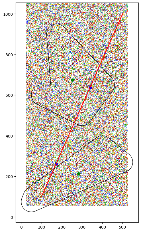
Projection des valeurs sur la polyligne

projected = analyze.project_onto(to_project, which='Max')

for vert in projected.myvertices:
    print(f"Projected point: {vert.x}, Value: {vert.y}")

Projected point: 177.37896754341685, Value: 9.999958038330078
Projected point: 587.6449711272588, Value: 9.999964714050293

fig, ax = plt.subplots(figsize=(10, 10))
a.plot_matplotlib(figax = (fig, ax))
analyze.polygons.plot_matplotlib(ax)
to_project.plot_matplotlib(ax)
ax.set_aspect('equal')

# Plot centroids
for poly in analyze.polygons.myvectors:
    ax.scatter(poly.centroid.x, poly.centroid.y, color='green', label='Centroids', s=50)

# Plot projected points
for vert in projected.myvertices:
    xy = to_project.linestring.interpolate(vert.x)
    ax.scatter(xy.x, xy.y, color='blue', label='Projected Points', s=50)