Multicriteria Analysis : smolt application

1. Import modules

import matplotlib.pyplot as plt
import shutil
import zipfile

from wolfhece.multicriteria.salmon import Smolt
from wolfhece.wolf_array import wolfpalette
from wolfhece.wolfresults_2D import views_2D, Wolfresults_2D

from wolfhece.pydownloader import toys_dataset

2. Access 2D results

# ------------------ Repository paths ------------------
# We download the simulation folder from wolf_examples repository,
# and we store it on our local machine.
zip_file_simulation= toys_dataset(dir= 'Simulation_CPU/example',
                                  file= 'Mery_18_Grid_025.zip',
                                  )
with zipfile.ZipFile(zip_file_simulation, 'r') as zip_ref:
    zip_ref.extractall(zip_file_simulation.parent)
simulation_folder = zip_file_simulation.parent / zip_file_simulation.stem

# We get the simulation file
sim_file_mery = simulation_folder / f"{simulation_folder.stem}"

assert sim_file_mery.is_file(),\
    f"The path {sim_file_mery} does not exist."

# ------------------ Data loading ------------------
# We read the simulated results
simulations = Wolfresults_2D(fname = sim_file_mery)

INFO:root:File C:\Users\pierre\Documents\Gitlab\HECEPython\wolfhece\data\downloads\Simulation_CPU\example\Mery_18_Grid_025.zip already exists. Skipping download.

3. Extract data from results

# We extract the variables of interest from the simulation as monoblock wolf arrays.
# We also set zero in mask.
TIME_STEP = -1 # Last one

array_velocity_norm = simulations.get_result(TIME_STEP, views_2D.UNORM, force_monoblock=True)
array_depth         = simulations.get_result(TIME_STEP, views_2D.WATERDEPTH, force_monoblock=True)
array_tke           = simulations.get_result(TIME_STEP, views_2D.KINETIC_ENERGY, force_monoblock=True)

INFO:root:Updating time steps information...
INFO:root:Time steps information updated.
INFO:root:Reading from results - step :77

4. Perform multicriteria analysis

# We perform the multicriteria analysis with the Smolt class.
smolt_analysis = Smolt(velocity = array_velocity_norm,
                       depth = array_depth,
                       tke = array_tke)

# We set  a wolfpalette to plot the results of the analysis.
values = [0, 1, 2, 3, 4, 4.00001]
colors = ["#FFFFFF","#7E7A7A","#AB0303","#FFFF00","#07DAFA","#07DAFA"]
palette = wolfpalette()
palette.set_discrete_values_colors(values, colors)

# We get and plot the result.
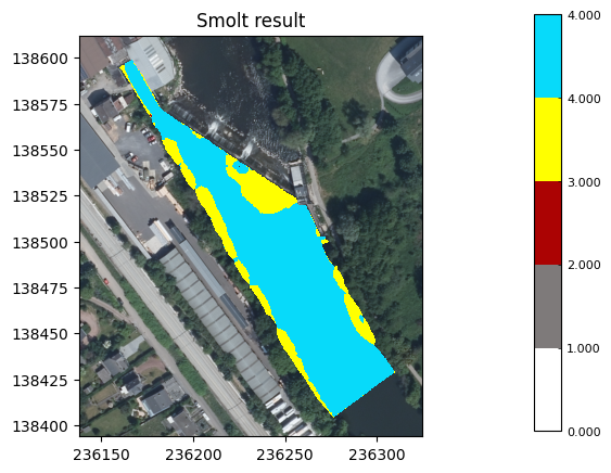
array = smolt_analysis.result
array.mypal = palette
print("\tResult: ","\n", "-"*50)
fig,ax = array.plot_matplotlib(Walonmap = True, update_palette = False, with_legend = True)
ax.set_title("Smolt result")
plt.show()


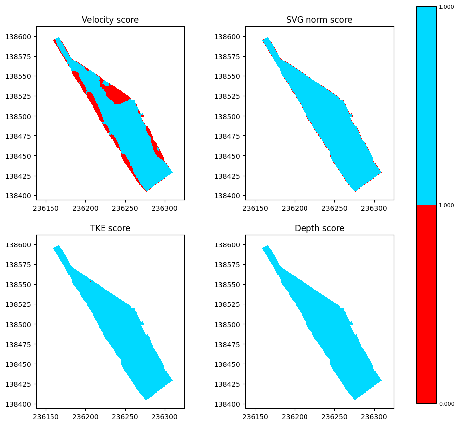
BACKGROUND = False
fig, axes = plt.subplots(2, 2, figsize=(10, 10))

# We investigate the scores of all the four variables used in the analysis.
velocity_score_figax = smolt_analysis.get_score_as_WolfArray('velocity').plot_matplotlib(update_palette = False,
                                                                                         with_legend = True,
                                                                                         Walonmap = BACKGROUND,
                                                                                         figax = (fig, axes[0,0]))
velocity_score_figax[1].set_title("Velocity score")

svg_score_figax = smolt_analysis.get_score_as_WolfArray('svg_norm').plot_matplotlib(update_palette = False,
                                                                                    with_legend = False,
                                                                                    Walonmap = BACKGROUND,
                                                                                    figax = (fig, axes[0,1]))
svg_score_figax[1].set_title("SVG norm score")

tke_score_figax = smolt_analysis.get_score_as_WolfArray('tke').plot_matplotlib(update_palette = False,
                                                                               with_legend = False,
                                                                               Walonmap = BACKGROUND,
                                                                               figax = (fig, axes[1,0]))
tke_score_figax[1].set_title("TKE score")

depth_score_figax = smolt_analysis.get_score_as_WolfArray('depth').plot_matplotlib(update_palette = False,
                                                                                   with_legend = False,
                                                                                   Walonmap = BACKGROUND,
                                                                                   figax = (fig, axes[1,1]))
depth_score_figax[1].set_title("Depth score")
plt.show()

WARNING:root:No weight provided. Setting weight to equal distribution.
WARNING:root:No weight provided. Setting weight to equal distribution.

        Result:
 --------------------------------------------------

5. Clean-up the example directory

shutil.rmtree(simulation_folder)