Eikonal Solver — Full Demonstration
This notebook illustrates the different variants of the Fast Marching Method (FMM) solver implemented in wolfhece.eikonal:
Isotropic 1st order vs 2nd order — spatial accuracy
Anisotropic 4-connected vs 8-connected (Ordered Upwind Method) — ability to capture oblique directions
Non-trivial application — anisotropic propagation with spatially variable speed field (wind over terrain)
Theoretical Background
The eikonal equation computes the arrival time \(T(\mathbf{x})\) of a front propagating from sources:
Isotropic: \(|\nabla T| = 1 / s(\mathbf{x})\) (scalar speed \(s\))
Anisotropic: \((\nabla T)^T \, D \, (\nabla T) = 1\) (metric tensor \(D\))
where \(D = R(\theta) \, \text{diag}(s_{\max}^2, s_{\min}^2) \, R(\theta)^T\) encodes a speed ellipse.
[1]:
import numpy as np
import matplotlib.pyplot as plt
from matplotlib.colors import Normalize

from wolfhece.eikonal import (
    _solve_eikonal_with_data,
    _solve_eikonal_with_data_second_order,
    _solve_eikonal_anisotropic,
    _solve_eikonal_anisotropic_4conn,
)
Common Utilities
[16]:
def make_isotropic_grid(n, speed=1.0):
    """Create an n×n domain with uniform speed (no border sources)."""
    mask = np.ones((n, n), dtype=np.float64)
    base = np.full((n, n), 10.0)   # arbitrary data for propagation
    test = np.full((n, n), -np.inf)  # never filters
    spd  = np.full((n, n), speed)
    return mask, base, test, spd


def make_anisotropic_grid(n):
    """Create an n×n domain with no border sources."""
    mask = np.ones((n, n), dtype=np.float64)
    return mask


def build_metric_tensor(n, s_max, s_min, theta):
    """Build the tensor D = R(θ) diag(s_max², s_min²) R(θ)^T.

    Physical convention: x = columns, y = rows.
    θ = 0 => fast direction along columns (x).
    """
    c, s = np.cos(theta), np.sin(theta)
    Dxx = np.full((n, n), (s_max * c)**2 + (s_min * s)**2)
    Dxy = np.full((n, n), (s_max**2 - s_min**2) * c * s)
    Dyy = np.full((n, n), (s_max * s)**2 + (s_min * c)**2)
    return Dxx, Dxy, Dyy
1. Isotropic: 1st Order vs 2nd Order
The standard FMM solver uses a 1st-order upwind finite difference scheme (error \(O(h)\)). The Sethian (1999) scheme uses a 2nd-order approximation when two consecutive upwind neighbours are available:
We compare both on a point source: the analytical solution is \(T = d / s\) along the axes.
[17]:
n = 101
c = n // 2
speed = 1.0

# --- 1st-order solver ---
mask1, base1, test1, spd1 = make_isotropic_grid(n, speed)
mask1[c, c] = 0.0
T1 = _solve_eikonal_with_data([(c, c)], mask1, base1, test1, spd1, 1.0, 1.0)

# --- 2nd-order solver ---
mask2, base2, test2, spd2 = make_isotropic_grid(n, speed)
mask2[c, c] = 0.0
T2 = _solve_eikonal_with_data_second_order([(c, c)], mask2, base2, test2, spd2, 1.0, 1.0)
[18]:
# Comparison along the diagonal
# Stay away from the domain edges to avoid boundary effects
max_d = c // 2
diag_range = np.arange(1, max_d)
exact_diag = diag_range * np.sqrt(2.0) / speed

t1_diag = np.array([T1[c + d, c + d] for d in diag_range])
t2_diag = np.array([T2[c + d, c + d] for d in diag_range])

err1 = np.abs(t1_diag - exact_diag)
err2 = np.abs(t2_diag - exact_diag)

fig, axes = plt.subplots(1, 3, figsize=(16, 4.5))

# T map (1st order)
im = axes[0].imshow(T1, cmap='inferno', origin='lower')
axes[0].set_title('T — 1st order')
axes[0].plot(c, c, 'w+', ms=12, mew=2)
plt.colorbar(im, ax=axes[0], shrink=0.8)

# T map (2nd order)
im2 = axes[1].imshow(T2, cmap='inferno', origin='lower')
axes[1].set_title('T — 2nd order')
axes[1].plot(c, c, 'w+', ms=12, mew=2)
plt.colorbar(im2, ax=axes[1], shrink=0.8)

# Error along the diagonal
axes[2].semilogy(diag_range, err1, 'o-', ms=3, label='1st order')
axes[2].semilogy(diag_range, err2, 's-', ms=3, label='2nd order')
axes[2].set_xlabel('Distance (cells)')
axes[2].set_ylabel('|T − T_exact|')
axes[2].set_title('Error along the diagonal')
axes[2].legend()
axes[2].grid(True, alpha=0.3)

fig.tight_layout()
plt.show()

print(f"Max diagonal error — 1st order: {err1.max():.4f}")
print(f"Max diagonal error — 2nd order: {err2.max():.4f}")
print(f"Improvement factor: {err1.max() / err2.max():.1f}×")
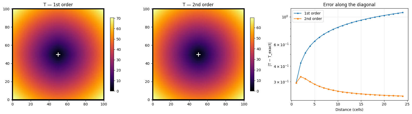
Max diagonal error — 1st order: 1.0809
Max diagonal error — 2nd order: 0.3289
Improvement factor: 3.3×
[19]:
# Comparison along the cardinal axis (theoretically zero error)
t1_axis = np.array([T1[c + d, c] for d in diag_range])
t2_axis = np.array([T2[c + d, c] for d in diag_range])
exact_axis = diag_range / speed

err1_ax = np.abs(t1_axis - exact_axis)
err2_ax = np.abs(t2_axis - exact_axis)

fig, ax = plt.subplots(figsize=(8, 4))
ax.semilogy(diag_range, err1_ax + 1e-16, 'o-', ms=3, label='1st order (cardinal axis)')
ax.semilogy(diag_range, err2_ax + 1e-16, 's-', ms=3, label='2nd order (cardinal axis)')
ax.semilogy(diag_range, err1, '^-', ms=3, alpha=0.5, label='1st order (diagonal)')
ax.semilogy(diag_range, err2, 'v-', ms=3, alpha=0.5, label='2nd order (diagonal)')
ax.set_xlabel('Distance (cells)')
ax.set_ylabel('|T − T_exact|')
ax.set_title('Isotropic error: cardinal axis vs diagonal')
ax.legend()
ax.grid(True, alpha=0.3)
plt.tight_layout()
plt.show()
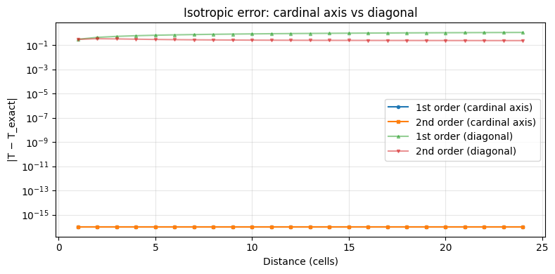
Isotropic Observations
Along the cardinal axis, both schemes are quasi-exact (error is at machine precision).
Along the diagonal, the 1st-order scheme overestimates \(T\) by a nearly constant amount (~6% for a square grid). The 2nd-order scheme significantly reduces this error.
The 2nd-order advantage is most pronounced far from the source, where two consecutive upwind neighbours are available.
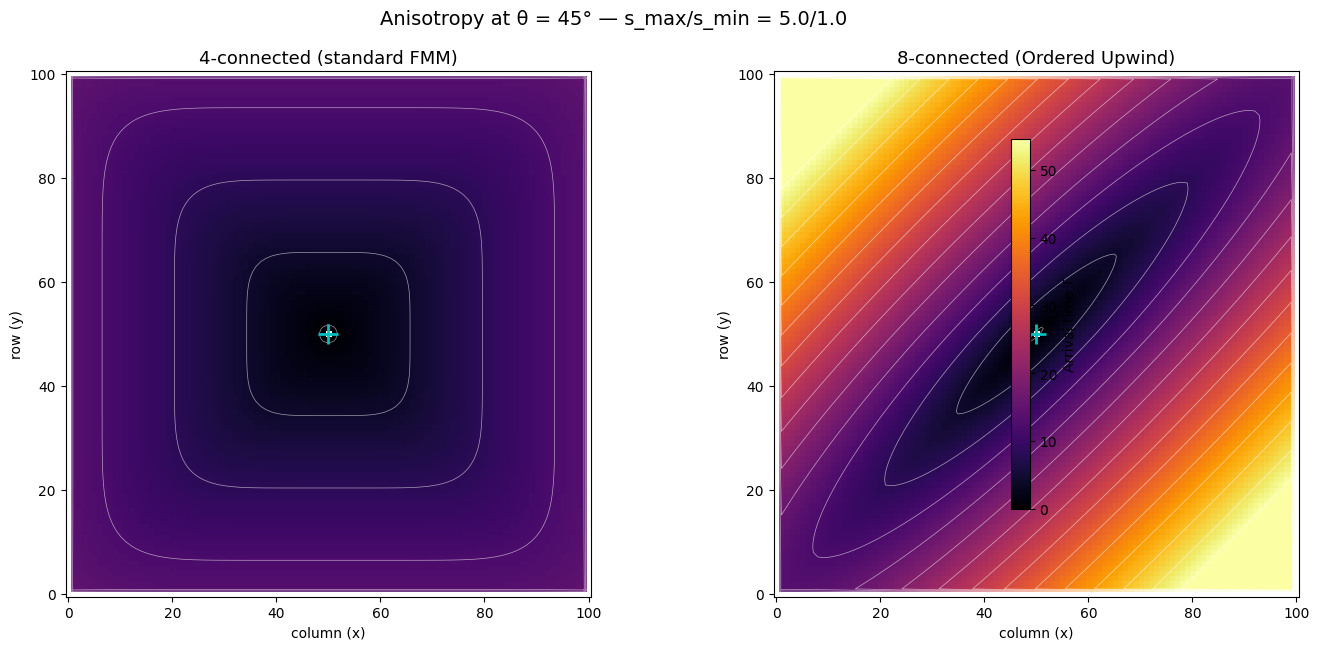
2. Anisotropic: 4-Connected vs 8-Connected (Ordered Upwind Method)
The 4-connected stencil only considers cardinal neighbours (N, S, E, W). When the fast direction is at \(\theta = 45°\), we have \(D_{xx} = D_{yy}\) and the cross-term \(D_{xy}\) cannot influence the solution — both diagonals have the same arrival time.
The 8-connected stencil (Sethian & Vladimirsky, 2003) considers all 8 neighbours and forms triangles for each adjacent pair. This allows solving the equation in oblique directions by fully exploiting the metric tensor.
[20]:
n = 101
c = n // 2
s_max, s_min = 5.0, 1.0
theta = np.pi / 4   # fast direction at 45°

# No T=0 border: only the central source is fixed
# (the solver handles domain boundaries via index checking)

# --- 4-connected solver ---
mask_4 = np.ones((n, n), dtype=np.float64)
Dxx, Dxy, Dyy = build_metric_tensor(n, s_max, s_min, theta)
mask_4[c, c] = 0.0
T_4conn = _solve_eikonal_anisotropic_4conn(
    [(c, c)], mask_4, Dxx.copy(), Dxy.copy(), Dyy.copy(), 1.0, 1.0)

# --- 8-connected solver (OUM) ---
mask_8 = np.ones((n, n), dtype=np.float64)
Dxx, Dxy, Dyy = build_metric_tensor(n, s_max, s_min, theta)
mask_8[c, c] = 0.0
T_8conn = _solve_eikonal_anisotropic(
    [(c, c)], mask_8, Dxx, Dxy, Dyy, 1.0, 1.0)
[21]:
# Mask T=0 cells for better visualisation
T_4plot = T_4conn.copy()
T_8plot = T_8conn.copy()
T_4plot[T_4plot == 0] = np.nan
T_8plot[T_8plot == 0] = np.nan

vmax = np.nanpercentile(T_8plot, 95)
levels = np.linspace(0.5, vmax, 15)

fig, axes = plt.subplots(1, 2, figsize=(14, 6))

for ax, T, title in [(axes[0], T_4plot, '4-connected (standard FMM)'),
                      (axes[1], T_8plot, '8-connected (Ordered Upwind)')]:
    im = ax.imshow(T, cmap='inferno', origin='lower',
                   norm=Normalize(vmin=0, vmax=vmax))
    # Iso-contours
    T_for_contour = np.where(np.isnan(T), 0, T)
    ax.contour(T_for_contour, levels=levels, colors='white', linewidths=0.5, alpha=0.6)
    ax.plot(c, c, 'c+', ms=15, mew=2)
    ax.set_title(title, fontsize=13)
    ax.set_xlabel('column (x)')
    ax.set_ylabel('row (y)')

plt.colorbar(im, ax=axes, shrink=0.8, label='Arrival time T')

fig.suptitle(f'Anisotropy at θ = 45° — s_max/s_min = {s_max}/{s_min}',
             fontsize=14, y=1.02)
fig.tight_layout()
plt.show()
C:\Users\pierre\AppData\Local\Temp\ipykernel_68240\1126657132.py:28: UserWarning: This figure includes Axes that are not compatible with tight_layout, so results might be incorrect.
  fig.tight_layout()
[22]:
# Profiles along the diagonals
# Limit distance to stay far from domain edges
# For the anti-diagonal (c+d, c-d), we need c-d > margin
max_d = c // 3  # ~16 cells, always > 30 cells from the edge
d_range = np.arange(1, max_d + 1)
dist_diag = d_range * np.sqrt(2.0)  # Euclidean distance

# SE diagonal (+i, +j) = fast direction for θ=45°
t4_fast = [T_4conn[c + d, c + d] for d in d_range]
t8_fast = [T_8conn[c + d, c + d] for d in d_range]

# NE anti-diagonal (+i, -j) = slow direction for θ=45°
t4_slow = [T_4conn[c + d, c - d] for d in d_range]
t8_slow = [T_8conn[c + d, c - d] for d in d_range]

fig, axes = plt.subplots(1, 2, figsize=(14, 5))

axes[0].plot(dist_diag, t4_fast, 'b--', label='4-conn: fast diag', lw=2)
axes[0].plot(dist_diag, t4_slow, 'r--', label='4-conn: slow diag', lw=2)
axes[0].plot(dist_diag, t8_fast, 'b-',  label='8-conn: fast diag', lw=2)
axes[0].plot(dist_diag, t8_slow, 'r-',  label='8-conn: slow diag', lw=2)
axes[0].set_xlabel('Euclidean distance')
axes[0].set_ylabel('Arrival time T')
axes[0].set_title('T along the diagonals')
axes[0].legend()
axes[0].grid(True, alpha=0.3)

# Slow / fast diagonal ratio
ratio_4 = np.array(t4_slow) / np.array(t4_fast)
ratio_8 = np.array(t8_slow) / np.array(t8_fast)
axes[1].plot(dist_diag, ratio_4, 'g--', label='4-conn', lw=2)
axes[1].plot(dist_diag, ratio_8, 'g-',  label='8-conn (OUM)', lw=2)
axes[1].axhline(s_max / s_min, color='gray', ls=':', label=f'theoretical ratio = {s_max/s_min}')
axes[1].set_xlabel('Euclidean distance')
axes[1].set_ylabel('T_slow / T_fast')
axes[1].set_title('Captured anisotropy ratio')
axes[1].legend()
axes[1].grid(True, alpha=0.3)

fig.tight_layout()
plt.show()

print(f"4-connected: slow/fast ratio = {ratio_4[-1]:.3f}  (expected ≈ {s_max/s_min:.1f})")
print(f"8-connected: slow/fast ratio = {ratio_8[-1]:.3f}  (expected ≈ {s_max/s_min:.1f})")
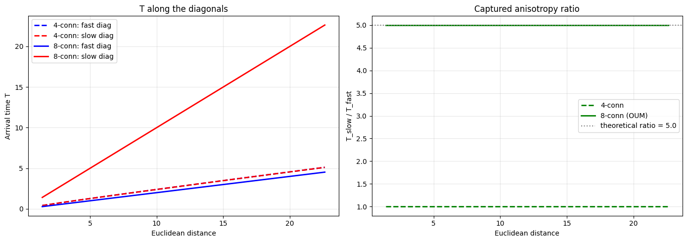
4-connected: slow/fast ratio = 1.000  (expected ≈ 5.0)
8-connected: slow/fast ratio = 5.000  (expected ≈ 5.0)
Anisotropic Observations
4-connected: the iso-contours are nearly identical squares in both diagonal directions. The slow/fast ratio is ~1.0 — the stencil cannot distinguish diagonals when \(D_{xx} = D_{yy}\).
8-connected (OUM): the iso-contours are ellipses oriented at 45°. The slow/fast ratio approaches the theoretical value \(s_{\max}/s_{\min}\).
The OUM method uses triangle updates between pairs of adjacent neighbours, which allows the front to propagate correctly in oblique directions.
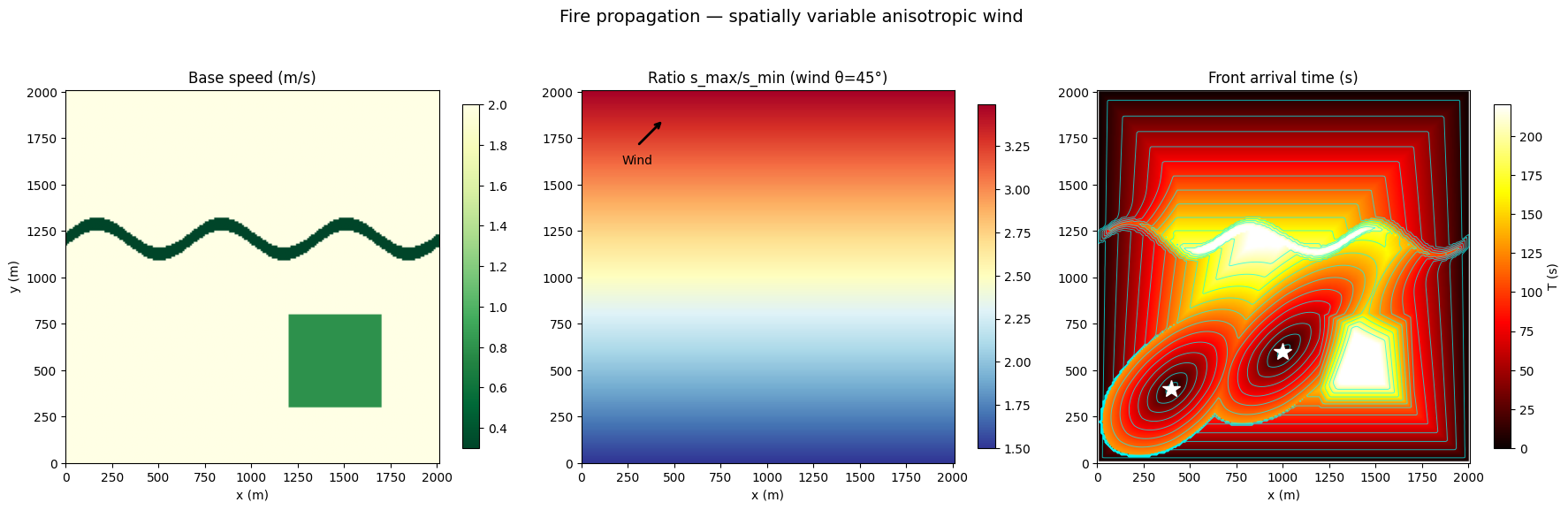
3. Non-trivial Application: Fire Propagation Under Wind
We simulate the propagation of a front (fire, pollutant, etc.) on a domain where:
The wind blows from SW to NE (\(\theta = 45°\)), accelerating propagation in that direction.
The base speed varies spatially (terrain with slow zones: river, dense forest).
The anisotropy is moderate (\(s_{\max}/s_{\min} = 3\)) and spatially variable (wind intensifies towards the north).
Two fire sources are placed and the propagation front is visualised.
[23]:
n = 201
dx = dy = 10.0  # 10 m cell size

# --- Base speed (scalar, spatially variable) ---
np.random.seed(42)
base_speed = 2.0 * np.ones((n, n))

# Sinusoidal river (slow band, E-W axis)
for j in range(n):
    river_i = int(n * 0.6 + 8 * np.sin(2 * np.pi * j / n * 3))
    i_lo = max(0, river_i - 3)
    i_hi = min(n, river_i + 4)
    base_speed[i_lo:i_hi, j] = 0.3  # water = very slow propagation

# Dense forest (square patch)
base_speed[30:80, 120:170] = 0.8

# --- Anisotropy: wind from SW to NE ---
theta_wind = np.pi / 4  # wind direction (45°)

# Anisotropy ratio increases northward (stronger wind at higher altitude)
row_idx = np.arange(n).reshape(-1, 1)
s_max_field = base_speed * (1.5 + 2.0 * row_idx / n)  # 1.5 → 3.5 × base_speed
s_min_field = base_speed * np.ones((n, n))             # base speed perpendicular to wind

# Build tensor D cell by cell
c_t = np.cos(theta_wind)
s_t = np.sin(theta_wind)
Dxx = (s_max_field * c_t)**2 + (s_min_field * s_t)**2
Dxy = (s_max_field**2 - s_min_field**2) * c_t * s_t
Dyy = (s_max_field * s_t)**2 + (s_min_field * c_t)**2

# --- Domain ---
mask = np.ones((n, n), dtype=np.float64)
mask[0, :] = 0;  mask[-1, :] = 0
mask[:, 0] = 0;  mask[:, -1] = 0

# Two fire sources
sources = [(40, 40), (60, 100)]
for si, sj in sources:
    mask[si, sj] = 0.0

# --- Solve ---
T_fire = _solve_eikonal_anisotropic(sources, mask, Dxx, Dxy, Dyy, dx, dy)

print(f"Domain: {n}×{n} = {n*dx:.0f} m × {n*dy:.0f} m")
print(f"Max arrival time: {T_fire[1:-1, 1:-1].max():.1f} s")
Domain: 201×201 = 2010 m × 2010 m
Max arrival time: 303.9 s
[24]:
fig, axes = plt.subplots(1, 3, figsize=(18, 5.5))

# 1) Base speed map
im0 = axes[0].imshow(base_speed, cmap='YlGn_r', origin='lower',
                      extent=[0, n*dx, 0, n*dy])
axes[0].set_title('Base speed (m/s)', fontsize=12)
axes[0].set_xlabel('x (m)')
axes[0].set_ylabel('y (m)')
plt.colorbar(im0, ax=axes[0], shrink=0.8)

# 2) Anisotropy ratio
aniso_ratio = s_max_field / np.maximum(s_min_field, 1e-6)
im1 = axes[1].imshow(aniso_ratio, cmap='RdYlBu_r', origin='lower',
                      extent=[0, n*dx, 0, n*dy])
axes[1].set_title(f'Ratio s_max/s_min (wind θ={int(np.degrees(theta_wind))}°)',
                   fontsize=12)
axes[1].set_xlabel('x (m)')
# Wind direction arrow
cx, cy = n*dx*0.15, n*dy*0.85
arrow_len = n*dx*0.1
axes[1].annotate('', xy=(cx + arrow_len*c_t, cy + arrow_len*s_t),
                  xytext=(cx, cy),
                  arrowprops=dict(arrowstyle='->', color='black', lw=2))
axes[1].text(cx, cy - n*dy*0.05, 'Wind', ha='center', fontsize=10)
plt.colorbar(im1, ax=axes[1], shrink=0.8)

# 3) Arrival time with iso-contours
T_plot = T_fire.copy()
T_plot[T_plot == 0] = np.nan
vmax_fire = np.nanpercentile(T_plot, 98)
im2 = axes[2].imshow(T_plot, cmap='hot', origin='lower',
                      extent=[0, n*dx, 0, n*dy],
                      norm=Normalize(vmin=0, vmax=vmax_fire))

# Temporal iso-contours
T_contour = np.where(np.isnan(T_plot), 0, T_plot)
x_coords = np.linspace(0, n*dx, n)
y_coords = np.linspace(0, n*dy, n)
contour_levels = np.linspace(vmax_fire * 0.05, vmax_fire * 0.9, 12)
axes[2].contour(x_coords, y_coords, T_contour, levels=contour_levels,
                colors='cyan', linewidths=0.7, alpha=0.7)

# Mark fire sources
for si, sj in sources:
    axes[2].plot(sj * dx, si * dy, 'w*', ms=15, mew=1)

axes[2].set_title('Front arrival time (s)', fontsize=12)
axes[2].set_xlabel('x (m)')
plt.colorbar(im2, ax=axes[2], shrink=0.8, label='T (s)')

fig.suptitle('Fire propagation — spatially variable anisotropic wind',
             fontsize=14, y=1.02)
fig.tight_layout()
plt.show()
[25]:
# Comparison with an equivalent isotropic solver
# (scalar speed = geometric mean √(s_max·s_min) )
s_iso = np.sqrt(s_max_field * s_min_field)
Dxx_iso = s_iso**2
Dxy_iso = np.zeros((n, n))
Dyy_iso = s_iso**2

mask_iso = np.ones((n, n), dtype=np.float64)
mask_iso[0, :] = 0;  mask_iso[-1, :] = 0
mask_iso[:, 0] = 0;  mask_iso[:, -1] = 0
for si, sj in sources:
    mask_iso[si, sj] = 0.0

T_iso = _solve_eikonal_anisotropic(sources, mask_iso, Dxx_iso, Dxy_iso, Dyy_iso, dx, dy)

# Difference
T_diff = T_fire - T_iso
T_diff[T_fire == 0] = np.nan

fig, axes = plt.subplots(1, 3, figsize=(18, 5))

vmax_comp = np.nanpercentile(np.abs(T_plot[~np.isnan(T_plot)]), 95)

for ax, T, title in [(axes[0], T_fire, 'Anisotropic (wind)'),
                      (axes[1], T_iso, 'Isotropic (mean speed)')]:
    Tp = T.copy()
    Tp[Tp == 0] = np.nan
    ax.imshow(Tp, cmap='hot', origin='lower',
              extent=[0, n*dx, 0, n*dy],
              norm=Normalize(vmin=0, vmax=vmax_fire))
    Tc = np.where(np.isnan(Tp), 0, Tp)
    ax.contour(x_coords, y_coords, Tc, levels=contour_levels,
               colors='cyan', linewidths=0.5, alpha=0.6)
    for si, sj in sources:
        ax.plot(sj * dx, si * dy, 'w*', ms=12)
    ax.set_title(title, fontsize=12)
    ax.set_xlabel('x (m)')

# Difference map
vabs = np.nanpercentile(np.abs(T_diff), 95)
im3 = axes[2].imshow(T_diff, cmap='RdBu_r', origin='lower',
                      extent=[0, n*dx, 0, n*dy],
                      norm=Normalize(vmin=-vabs, vmax=vabs))
axes[2].set_title('ΔT = T_aniso − T_iso', fontsize=12)
axes[2].set_xlabel('x (m)')
plt.colorbar(im3, ax=axes[2], shrink=0.8, label='ΔT (s)')

fig.suptitle('Impact of anisotropy on arrival time', fontsize=14, y=1.02)
fig.tight_layout()
plt.show()

print(f"Mean ΔT = {np.nanmean(T_diff):+.1f} s")
print(f"Max ΔT  = {np.nanmax(T_diff):+.1f} s (max delay: downwind zone)")
print(f"Min ΔT  = {np.nanmin(T_diff):+.1f} s (max advance: upwind zone)")
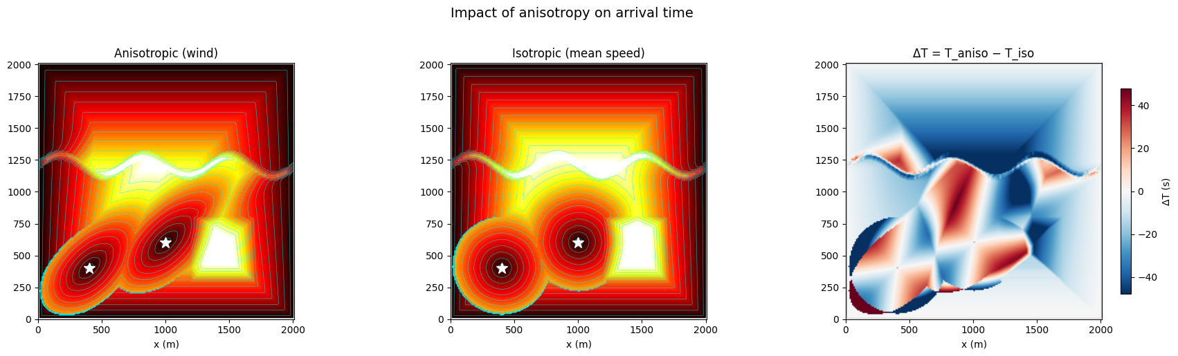
Mean ΔT = -10.9 s
Max ΔT  = +124.8 s (max delay: downwind zone)
Min ΔT  = -131.3 s (max advance: upwind zone)
Observations — Non-trivial Case
The wind accelerates propagation in the NE quadrant (negative \(\Delta T\)) and slows it down in the SW quadrant.
The river acts as a partial firebreak: the base speed drops to 0.3 m/s, creating a visible local delay.
The spatially variable anisotropy (increasing ratio towards the north) elongates the iso-time ellipses in the upper part of the domain.
Two fire sources: the fronts merge, and the arrival time is the minimum of both propagations (Huygens’ principle).
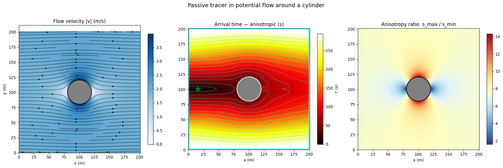
4. Application: Passive Tracer in a Flow Around an Obstacle
We simulate the advection-diffusion of a passive tracer (e.g., a pollutant dye) released upstream of a circular obstacle in a 2D potential flow.
Physical model:
The velocity field \(\mathbf{v}(x,y)\) is the irrotational potential flow around a cylinder of radius \(R\).
The tracer is transported by advection (carried by the flow) and spreads by diffusion (turbulent/molecular).
In a direction \(\hat{n}\), the effective front speed is approximated as:
\[s(\hat{n}) \approx |\mathbf{v} \cdot \hat{n}| + \kappa\]where \(\kappa\) is the isotropic diffusion speed.
Metric tensor construction: At each cell, the local flow direction \(\alpha = \text{atan2}(v, u)\) gives the fast axis orientation, and:
\(s_{\max} = |\mathbf{v}| + \kappa\) — speed along the flow (fast axis)
\(s_{\min} = \kappa\) — speed perpendicular to the flow (slow axis)
The Péclet number \(\text{Pe} = U_\infty / \kappa\) characterises the advection/diffusion ratio.
Note: The eikonal tensor is symmetric, so it gives the same speed upstream and downstream along the flow axis. This approximation is accurate for the downstream front but overestimates upstream propagation.
[30]:
# --- Domain ---
n_t = 201
dx_t = dy_t = 1.0  # 1 m cells

# Potential flow parameters
U_inf = 2.0    # free-stream velocity (m/s), flows along +x
R_cyl = 20.0   # cylinder radius (m)
kappa = 0.3    # turbulent diffusion speed (m/s)

# Grid coordinates (cell centres)
x_t = (np.arange(n_t) + 0.5) * dx_t
y_t = (np.arange(n_t) + 0.5) * dy_t
X_t, Y_t = np.meshgrid(x_t, y_t)

# Cylinder centre
x0_cyl = n_t * dx_t / 2
y0_cyl = n_t * dy_t / 2

# Coordinates relative to cylinder centre
Xc_t = X_t - x0_cyl
Yc_t = Y_t - y0_cyl
r2_t = np.maximum(Xc_t**2 + Yc_t**2, 1e-10)

# --- Potential flow velocity (u, v) ---
u_flow = U_inf * (1 - R_cyl**2 * (Xc_t**2 - Yc_t**2) / r2_t**2)
v_flow = -U_inf * R_cyl**2 * 2 * Xc_t * Yc_t / r2_t**2

# Inside the cylinder: zero velocity
inside_cyl = (Xc_t**2 + Yc_t**2) <= R_cyl**2
u_flow[inside_cyl] = 0.0
v_flow[inside_cyl] = 0.0

# Velocity magnitude and direction
V_mag = np.sqrt(u_flow**2 + v_flow**2)
theta_flow = np.arctan2(v_flow, u_flow)

# --- Metric tensor: fast axis = flow direction ---
s_max_t = V_mag + kappa                        # along flow (fast)
s_min_t = np.full((n_t, n_t), kappa)           # perpendicular (slow)

c_f = np.cos(theta_flow)
s_f = np.sin(theta_flow)
Dxx_t = (s_max_t * c_f)**2 + (s_min_t * s_f)**2
Dxy_t = (s_max_t**2 - s_min_t**2) * c_f * s_f
Dyy_t = (s_max_t * s_f)**2 + (s_min_t * c_f)**2

# --- Mask: only cylinder interior and tracer source are frozen (T=0) ---
# No border sources — borders are regular cells that will be reached by the front.
mask_t = np.ones((n_t, n_t), dtype=np.float64)
mask_t[inside_cyl] = 0  # impermeable obstacle

# Tracer source: upstream, centred vertically
src_tracer = [(n_t // 2, 15)]
mask_t[src_tracer[0][0], src_tracer[0][1]] = 0.0

# --- Solve ---
T_tracer = _solve_eikonal_anisotropic(src_tracer, mask_t, Dxx_t, Dxy_t, Dyy_t, dx_t, dy_t)

# Valid cells: finite T, excluding source (T=0) and cylinder interior
valid_t = np.isfinite(T_tracer) & (T_tracer > 0) & ~inside_cyl
print(f"Domain: {n_t}×{n_t} = {n_t*dx_t:.0f} m × {n_t*dy_t:.0f} m")
print(f"Cylinder: R = {R_cyl:.0f} m, centre = ({x0_cyl:.0f}, {y0_cyl:.0f})")
print(f"Free-stream velocity: U∞ = {U_inf:.1f} m/s")
print(f"Diffusion speed: κ = {kappa:.1f} m/s  (Pe ≈ {U_inf/kappa:.0f})")
print(f"Max arrival time: {T_tracer[valid_t].max():.1f} s")
Domain: 201×201 = 201 m × 201 m
Cylinder: R = 20 m, centre = (100, 100)
Free-stream velocity: U∞ = 2.0 m/s
Diffusion speed: κ = 0.3 m/s  (Pe ≈ 7)
Max arrival time: 317.6 s
[31]:
fig, axes = plt.subplots(1, 3, figsize=(18, 5.5))
extent_t = [0, n_t * dx_t, 0, n_t * dy_t]
theta_c = np.linspace(0, 2 * np.pi, 100)
cyl_x = x0_cyl + R_cyl * np.cos(theta_c)
cyl_y = y0_cyl + R_cyl * np.sin(theta_c)

# 1) Velocity magnitude + streamlines
im_v = axes[0].imshow(V_mag, cmap='Blues', origin='lower', extent=extent_t)
axes[0].streamplot(x_t, y_t, u_flow, v_flow,
                   color='black', density=1.2, linewidth=0.6, arrowsize=0.8)
axes[0].fill(cyl_x, cyl_y, color='gray', ec='black', lw=1.5, zorder=5)
axes[0].set_title('Flow velocity |v| (m/s)', fontsize=12)
axes[0].set_xlabel('x (m)');  axes[0].set_ylabel('y (m)')
axes[0].set_aspect('equal')
plt.colorbar(im_v, ax=axes[0], shrink=0.8)

# 2) Anisotropic arrival time with iso-contours
T_plot_t = T_tracer.copy()
T_plot_t[T_plot_t == 0] = np.nan
T_plot_t[inside_cyl] = np.nan
vmax_t = np.nanpercentile(T_plot_t, 95)
im_t = axes[1].imshow(T_plot_t, cmap='hot', origin='lower', extent=extent_t,
                       norm=Normalize(vmin=0, vmax=vmax_t))
T_cont_t = np.where(np.isnan(T_plot_t), 0, T_plot_t)
levels_t = np.linspace(vmax_t * 0.05, vmax_t * 0.9, 15)
axes[1].contour(x_t, y_t, T_cont_t, levels=levels_t,
                colors='cyan', linewidths=0.7, alpha=0.7)
axes[1].fill(cyl_x, cyl_y, color='gray', ec='white', lw=1.5, zorder=5)
axes[1].plot(x_t[src_tracer[0][1]], y_t[src_tracer[0][0]], 'g*', ms=15, mew=1)
axes[1].set_title('Arrival time — anisotropic (s)', fontsize=12)
axes[1].set_xlabel('x (m)')
axes[1].set_aspect('equal')
plt.colorbar(im_t, ax=axes[1], shrink=0.8, label='T (s)')

# 3) Anisotropy ratio
ratio_t = s_max_t / np.maximum(s_min_t, 1e-6)
ratio_t[inside_cyl] = np.nan
im_r = axes[2].imshow(ratio_t, cmap='RdYlBu_r', origin='lower', extent=extent_t)
axes[2].fill(cyl_x, cyl_y, color='gray', ec='black', lw=1.5, zorder=5)
axes[2].set_title('Anisotropy ratio  s_max / s_min', fontsize=12)
axes[2].set_xlabel('x (m)')
axes[2].set_aspect('equal')
plt.colorbar(im_r, ax=axes[2], shrink=0.8)

fig.suptitle('Passive tracer in potential flow around a cylinder',
             fontsize=14, y=1.02)
fig.tight_layout()
plt.show()
[32]:
# Isotropic comparison: scalar speed = geometric mean √(s_max · s_min)
s_geo_t = np.sqrt(s_max_t * s_min_t)
Dxx_geo = s_geo_t**2
Dxy_geo = np.zeros((n_t, n_t))
Dyy_geo = s_geo_t**2

mask_iso_t = np.ones((n_t, n_t), dtype=np.float64)
mask_iso_t[inside_cyl] = 0
mask_iso_t[src_tracer[0][0], src_tracer[0][1]] = 0.0

T_iso_t = _solve_eikonal_anisotropic(src_tracer, mask_iso_t,
                                      Dxx_geo, Dxy_geo, Dyy_geo, dx_t, dy_t)

# Difference
T_diff_t = T_tracer - T_iso_t
T_diff_t[T_tracer == 0] = np.nan
T_diff_t[inside_cyl] = np.nan

fig, axes = plt.subplots(1, 3, figsize=(18, 5))

for ax, T_arr, title in [(axes[0], T_tracer, 'Anisotropic (advection + diffusion)'),
                          (axes[1], T_iso_t, r'Isotropic ($\sqrt{s_{max} \cdot s_{min}}$)')]:
    Tp = T_arr.copy()
    Tp[Tp == 0] = np.nan
    Tp[inside_cyl] = np.nan
    ax.imshow(Tp, cmap='hot', origin='lower', extent=extent_t,
              norm=Normalize(vmin=0, vmax=vmax_t))
    Tc = np.where(np.isnan(Tp), 0, Tp)
    ax.contour(x_t, y_t, Tc, levels=levels_t,
               colors='cyan', linewidths=0.5, alpha=0.6)
    ax.fill(cyl_x, cyl_y, color='gray', ec='white', lw=1.5, zorder=5)
    ax.plot(x_t[src_tracer[0][1]], y_t[src_tracer[0][0]], 'g*', ms=12)
    ax.set_title(title, fontsize=12)
    ax.set_xlabel('x (m)')
    ax.set_aspect('equal')

# ΔT map
vabs_t = np.nanpercentile(np.abs(T_diff_t), 95)
im_d = axes[2].imshow(T_diff_t, cmap='RdBu_r', origin='lower', extent=extent_t,
                       norm=Normalize(vmin=-vabs_t, vmax=vabs_t))
axes[2].fill(cyl_x, cyl_y, color='gray', ec='black', lw=1.5, zorder=5)
axes[2].set_title('ΔT = T_aniso − T_iso (s)', fontsize=12)
axes[2].set_xlabel('x (m)')
axes[2].set_aspect('equal')
plt.colorbar(im_d, ax=axes[2], shrink=0.8, label='ΔT (s)')

fig.suptitle('Impact of flow direction on tracer arrival time', fontsize=14, y=1.02)
fig.tight_layout()
plt.show()

print(f"Mean ΔT = {np.nanmean(T_diff_t):+.1f} s")
print(f"Max ΔT  = {np.nanmax(T_diff_t):+.1f} s")
print(f"Min ΔT  = {np.nanmin(T_diff_t):+.1f} s")
C:\Users\pierre\AppData\Local\Temp\ipykernel_68240\408304828.py:15: RuntimeWarning: invalid value encountered in subtract
  T_diff_t = T_tracer - T_iso_t
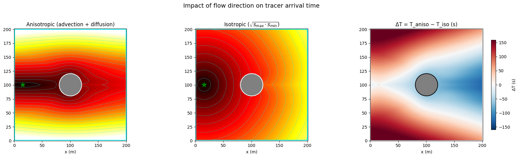
Mean ΔT = +34.7 s
Max ΔT  = +195.7 s
Min ΔT  = -125.5 s
Observations — Passive Tracer Advection
The anisotropic iso-contours are elongated downstream, following the streamlines around the obstacle. The tracer reaches the far side of the domain much faster along the flow direction than laterally.
The isotropic solver uses the geometric-mean speed \(\sqrt{s_{\max} \cdot s_{\min}}\) at each cell but ignores flow direction: the iso-contours are more circular and wrap symmetrically around the cylinder.
The \(\Delta T\) map reveals:
Negative values (blue) downstream of the source: the anisotropic model predicts faster arrival because advection carries the tracer along the flow axis.
Positive values (red) laterally and upstream of the obstacle: the anisotropic model predicts slower spreading where only diffusion operates (\(s_{\min} = \kappa\)).
The wake region behind the cylinder shows complex behaviour: the flow accelerates on the sides of the obstacle (\(|v| \to 2 U_\infty\)), creating preferential pathways.
Limitation: The symmetric tensor gives equal speed upstream and downstream along the flow axis. A more accurate model would require an asymmetric advection term \(\mathbf{v} \cdot \nabla T\).
Summary of Solver Variants
Solver |
Stencil |
Order |
Anisotropy |
Usage |
|---|---|---|---|---|
|
4-conn |
1st |
No |
Data inpainting |
|
4-conn |
2nd |
No |
High-precision inpainting |
|
4-conn |
1st |
Partial |
Comparison / debug |
|
8-conn OUM |
1st |
Full |
Anisotropic propagation |