Statistiques de données de pluie

Manipulation de données en provenance du site https://hydrometrie.wallonie.be

Import de modules

[7]:

import matplotlib.pyplot as plt
import numpy as np
import datetime as dt

from wolfhece import is_enough
if not is_enough('2.2.63'):
     print('Please update wolfhece to version 2.2.63 or higher to run this notebook')

from wolfhece.hydrometry.rain_SPWMI import *
from wolfhece.hydrometry.flow_SPWMI import *

Instanciation des objets

Les séries temporelles n’ont pas la même durée selon le pas d’acquisition.

Pour faciliter la manipulation, des classes spécifiques sont proposées pour les pas de 5 minutes et 1 heure.

[ ]:

#objet de gestion des pluvios SPW
precip_1h = SPW_pluviographs_1h()

Chargement de toutes les données

Une fois en local, le chargement de toutes les données ne prend que quelques secondes.

Le format parquet est particulièrement efficace dans ce cadre.

La routine “load_all” retourne un dictionnaire dont les clés sont les ts_id et les valeurs sont les séries pandas.

Ce dictionnaire est également disponible comme attribut de l’objet. L’accès à une station peut s’y faire grâce à son nom, la conversion vers le ts_id étant gérée pour vous.

[9]:

all_data = precip_1h.load_all()

print('Type of the data : {0}'.format(type(all_data)))

83it [00:01, 80.06it/s]WARNING:root:The file C:\Users\pierre\Documents\Gitlab\HECEPython\docs\source\tutorials\..\..\..\wolfhece\hydrometry\..\data\hydrometry\rain\1h\399076010.parquet is empty, unable to load data for station C:\Users\pierre\Documents\Gitlab\HECEPython\docs\source\tutorials\..\..\..\wolfhece\hydrometry\..\data\hydrometry\rain\1h\399076010.parquet
92it [00:01, 72.63it/s]WARNING:root:The file C:\Users\pierre\Documents\Gitlab\HECEPython\docs\source\tutorials\..\..\..\wolfhece\hydrometry\..\data\hydrometry\rain\1h\403325010.parquet is empty, unable to load data for station C:\Users\pierre\Documents\Gitlab\HECEPython\docs\source\tutorials\..\..\..\wolfhece\hydrometry\..\data\hydrometry\rain\1h\403325010.parquet
93it [00:01, 76.78it/s]

Type of the data : <class 'dict'>

Extraire des statistiques

[10]:

station = 'Jalhay'
stats = precip_1h.analyze(precip_1h[station], name=station)
# return a StatisticsSeries class
print(stats)
print(precip_1h['Jalhay'].index[-1])

Statistics for Jalhay:
Global stats: Mean: 0.14
Median: 0.00
Std: 0.60
Min: 0.00
Max: 28.30
Q25: 0.00
Q75: 0.00
Skewness: 11.08
Kurtosis: 223.96
Number of values: 211378
Total number of values: 211385
Coverage: 9999.67%
Missing values: Number: 7
Percentage: 0.33%
Date range: Start: 2002-01-01 00:00:00+01:00
End: 2026-02-11 16:00:00+01:00
All ranges: [(Timestamp('2002-01-01 00:00:00+0100', tz='pytz.FixedOffset(60)'), Timestamp('2006-03-01 13:00:00+0100', tz='pytz.FixedOffset(60)')), (Timestamp('2006-03-01 15:00:00+0100', tz='pytz.FixedOffset(60)'), Timestamp('2006-03-11 15:00:00+0100', tz='pytz.FixedOffset(60)')), (Timestamp('2006-03-11 17:00:00+0100', tz='pytz.FixedOffset(60)'), Timestamp('2006-03-13 09:00:00+0100', tz='pytz.FixedOffset(60)')), (Timestamp('2006-03-13 14:00:00+0100', tz='pytz.FixedOffset(60)'), Timestamp('2010-06-22 12:00:00+0100', tz='pytz.FixedOffset(60)')), (Timestamp('2010-06-22 14:00:00+0100', tz='pytz.FixedOffset(60)'), Timestamp('2026-02-11 16:00:00+0100', tz='pytz.FixedOffset(60)'))]
Years: Number of years: 25, Number of complete years: 23
2026-02-11 16:00:00+01:00

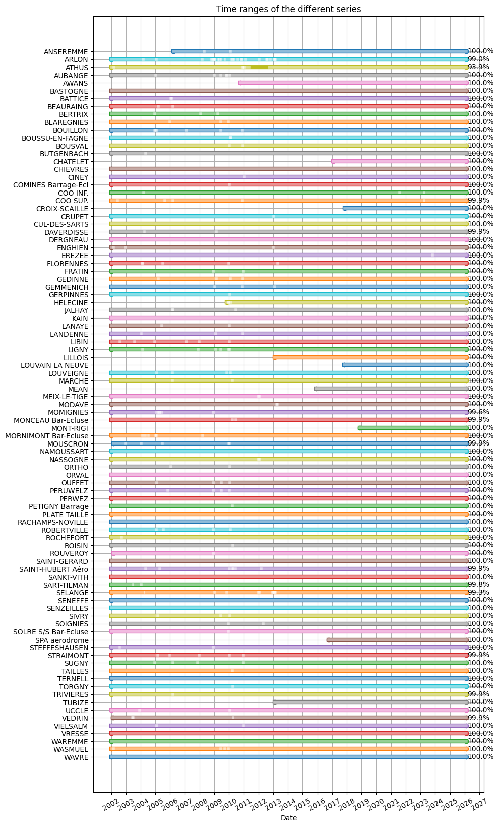
Tracer les périodes de données disponibles

[11]:

fig,ax = precip_1h.plot_time_ranges(precip_1h.analyze_all())
fig.set_size_inches(10,20)

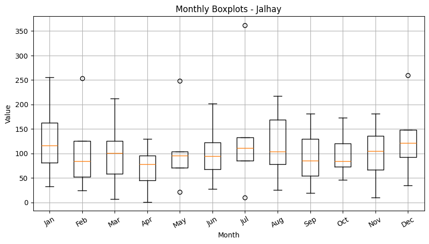
../_images/tutorials_stats_pluie_hydrometry_10_0.png

Evolution mensuelle

[12]:

precip_1h.plot_monthly_boxplots(stats)

[12]:

(<Figure size 1000x500 with 1 Axes>,
 <Axes: title={'center': 'Monthly Boxplots - Jalhay'}, xlabel='Month', ylabel='Value'>)

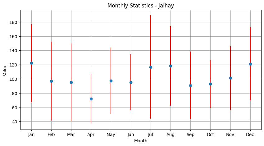
../_images/tutorials_stats_pluie_hydrometry_12_1.png

[13]:

precip_1h.plot_monthly_statistics(stats)

[13]:

(<Figure size 1000x500 with 1 Axes>,
 <Axes: title={'center': 'Monthly Statistics - Jalhay'}, xlabel='Month', ylabel='Value'>)

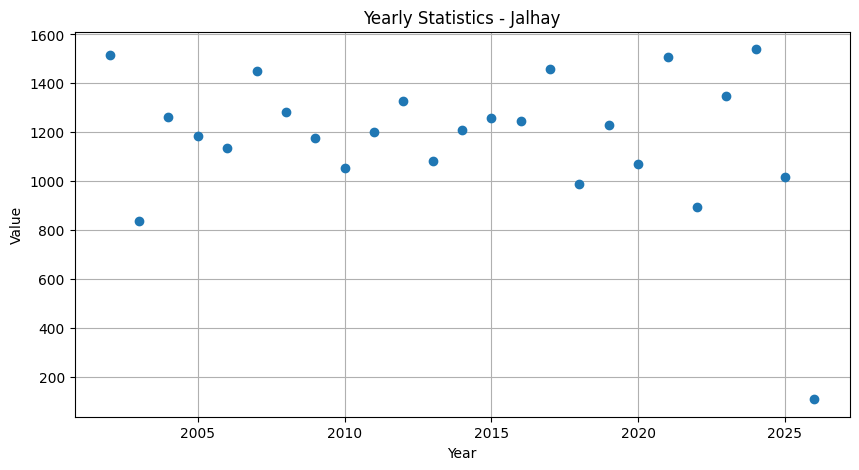
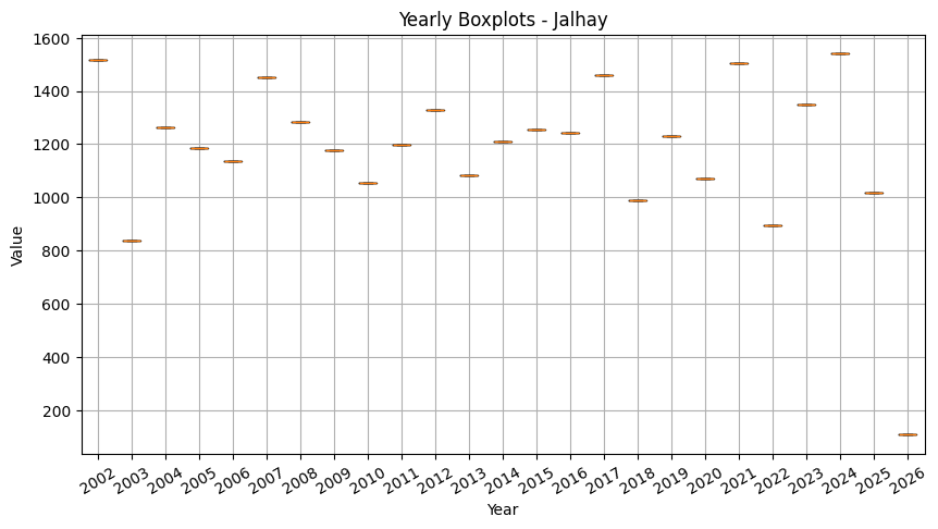
../_images/tutorials_stats_pluie_hydrometry_13_1.png

Evolution annuelle

[14]:

precip_1h.plot_yearly_boxplots(stats)

[14]:

(<Figure size 1000x500 with 1 Axes>,
 <Axes: title={'center': 'Yearly Boxplots - Jalhay'}, xlabel='Year', ylabel='Value'>)

../_images/tutorials_stats_pluie_hydrometry_15_1.png

[15]:

precip_1h.plot_yearly_statistics(stats)

[15]:

(<Figure size 1000x500 with 1 Axes>,
 <Axes: title={'center': 'Yearly Statistics - Jalhay'}, xlabel='Year', ylabel='Value'>)

../_images/tutorials_stats_pluie_hydrometry_16_1.png