WOLF 2D

Note

Mainly based on : Detailed Inundation Modelling Using High Resolution DEMs

Mathematical model

The flow model is based on the two-dimensional depth-averaged equations of volume and momentum conservation. In the “shallow-water” approach, it is basically assumed that velocities normal to the main flow plane are significantly smaller than those in this main flow direction. Consequently, the pressure field is almost hydrostatic everywhere.

The large majority of flows occurring in rivers, even highly transient, can reasonably be seen as shallow everywhere, except in the vicinity of some singularities (e.g. weirs). Indeed, vertical velocity components remain generally low compared to velocity components in the horizontal plane and, consequently, flows may be considered as mainly two-dimensional. Thus, the approach used in WOLF is suitable for many of the problems encountered in river management, and especially flood inundation mapping.

The conservative form of the depth-averaged equations of volume and momentum conservation can be written as follows, using vector notations:

(1)\[\frac{{\partial {\bf{s}}}}{{\partial t}} + \frac{{\partial {\bf{f}}}}{{\partial x}} + \frac{{\partial {\bf{g}}}}{{\partial y}} + \frac{{\partial {{\bf{f}}_{\rm{d}}}}}{{\partial x}} + \frac{{\partial {{\bf{g}}_{\rm{d}}}}}{{\partial y}} = {{\bf{S}}_0} - {{\bf{S}}_{\rm{f}}}\]

where \({\bf{s}} = {\left[ {\begin{array}{\*{20}{c}} h&{hu}&{hv} \end{array}} \right]^{\rm{T}}}\) is the vector of the conservative unknowns. \(\bf{f}\) and \(\bf{g}\) represent the advective and pressure fluxes in directions \(x\) and \(y\), while \({\bf{f}}_{\rm{d}}\) and \({\bf{g}}_{\rm{d}}\) are the diffusive fluxes:

(2)\[\begin{split}{\bf{f}} = \left( {\begin{array}{*{20}{c}} {hu}\\ {h{u^2} + {\textstyle{1 \over 2}}g{h^2}}\\ {huv} \end{array}} \right)\end{split}\]

(3)\[\begin{split}{\bf{g}} = \left( {\begin{array}{*{20}{c}} {hv}\\ {huv}\\ {h{v^2} + {\textstyle{1 \over 2}}g{h^2}} \end{array}} \right)\end{split}\]

(4)\[\begin{split}{{\bf{f}}_{\rm{d}}} = - \frac{h}{\rho }\left( {\begin{array}{*{20}{c}} 0\\ {{\sigma _x}}\\ {{\tau _{xy}}} \end{array}} \right)\end{split}\]

(5)\[\begin{split}{{\bf{g}}_{\rm{d}}} = - \frac{h}{\rho }\left( {\begin{array}{*{20}{c}} 0\\ {{\tau _{xy}}}\\ {{\sigma _y}} \end{array}} \right)\end{split}\]

\({\bf{S}}_0\) and \({\bf{S}}_f\) designate respectively the bottom slope and the friction terms:

(6)\[{\bf{S}}_0 = - gh{\left[ {\begin{array}{*{20}{c}} 0& {\frac{\partial{z_b}}{\partial x}}& {\frac{\partial {z_b}} {\partial y}} \end{array}} \right]^{\rm{T}}}\]

(7)\[{\bf{S}}_\rm{f} = {\left[ {\begin{array}{\*{20}{c}} 0& {\tau _{\rm{b}x}} \frac{\Delta \Sigma}{\rho}& {\tau _{\rm{b}y}} \frac{\Delta\Sigma }{\rho} \end{array}} \right]^{\rm{T}}}\]

In Eq. (1) to (7), \(t\) is the time, \(x\) and \(y\) the space coordinates, \(h\) the water depth, \(ut\) and \(v\) the depth-averaged velocity components, \(z_b\) the bottom elevation, \(g\) the gravity acceleration, \(\rho\) the density of water, \(\tau _{bx}\) and \(\tau _{by}\) the bottom shear stresses, \(\sigma _x\) and \(\sigma _y\) the turbulent normal stresses, and \(\tau _{xy}\) the turbulent shear stress. Consistently with Hervouet (2003),

(8)\[\Delta \Sigma = \sqrt {1 + {{\left( {{\frac{\partial {z_{\rm{b}}}} {\partial x}}} \right)}^2} + {{\left( {{\frac{\partial {z_{\rm{b}}}} {\partial y}}} \right)}^2}}\]

can reproduce the increased friction area on an irregular (natural) topography (Dewals, 2006).

Friction modelling

The bottom friction is conventionally modelled with empirical laws, such as the Manning formula. The model enables the definition of a spatially distributed roughness coefficient to impact different land-uses, floodplain vegetations or sub-grid bed forms… In addition, the friction along side walls is reproduced through a process-oriented formulation developed by Dewals (2006). Finally, friction terms become:

(9)\[\frac{{{\tau _{{\rm{b}}x}}}}{\rho } = gh\;u\left[ {\sqrt {{u^2} + {v^2}} \frac{{n_{\rm{b}}^2}}{{{h^{4/3}}}} + u\sum\limits_{{k_x} = 1}^{{N_x}} {\frac{4}{3}\frac{{n_{\rm{w}}^2}}{{{h^{1/3}}{\kern 1pt} \Delta y}}} } \right]\]

and

(10)\[\frac{{{\tau _{{\rm{b}}y}}}}{\rho } = gh\;v\left[ {\sqrt {{u^2} + {v^2}} \frac{{n_{\rm{b}}^2}}{{{h^{4/3}}}} + v\sum\limits_{{k_y} = 1}^{{N_y}} {\frac{4}{3}\frac{{n_{\rm{w}}^{3/2}}}{{{h^{1/3}}\Delta x{\kern 1pt} }}} } \right]\]

where the Manning coefficient \({n_{\rm{b}}}\) and \({n_{\rm{w}}}\) characterize respectively the bottom and the side-walls roughness. These relations have been written for Cartesian grids, such as used in the present study.

The internal friction might be reproduced by applying a proper turbulence model. For SWE, various approaches are proposed in the literature, as rather simple algebraic expressions of turbulent viscosity (Fisher et al., 1979; Hervouet, 2003) or more complex mathematical models with 1 or 2 additional equations (Rastogi and Rodi, 1978; Rodi, 1984; Erpicum, 2006).

In WOLF2D, there are several formulations available to compute the turbulent shear stresses. The simplest one is the mixing length model with a constant turbulent viscosity. The most complex one is an original 2D k-epsilon model (Erpicum, 2006).

The bottom friction models available in WOLF2D (Fortran) are :

• Manning/Strickler

• Barr-Bathurst

• Colebrrok-White (fully semi-implicit or explicit)

• Bazin

• Haaland

• Hazen-Williams

Grid and numerical scheme

The solver includes a mesh generator and can deal with multiblock grids (Erpicum, 2006). Within each block, the grid is Cartesian to take advantage of the lower computation time and the gain in accuracy provided by this type of structured grids compared to unstructured ones.

The multiblock features increase the domain area which can be discretized with a constant cells number and enable local mesh refinements close to areas of interest. It is thus a solution to overcome the main drawback of Cartesian grid, i.e. the high number of cells needed for a fine enough discretization of complexes geometries. Moreover, it allows combining local high precision with strong computation speed requirements.

In addition, an automatic grid adaptation technique restricts the simulation domain to the wet cells to decrease the number of computational elements. An original iterative technique restores mass and momentum conservation at each step of meshes drying.

Eq. (1) is discretized in space with a finite volume scheme. This ensures a correct mass and momentum conservation, which is a must for handling properly discontinuous solutions such as moving hydraulic jumps. As a consequence, no assumption is required regarding the smoothness of the solution. Reconstruction at cells interfaces can be performed with a constant or linear approach. For the latter, together with slope limiting, a second-order spatial accuracy is obtained.

In a similar way, variables at the border between adjacent blocks are reconstructed linearly, using in addition ghost points as depicted in Fig. 1. The value of the variables at the ghost points is evaluated from the value of the subjacent cells. Moreover, to ensure conservation properties at the border between adjacent blocks and thus to compute accurate volume and momentum balances, fluxes related to the larger cells are computed at the level of the finer ones.

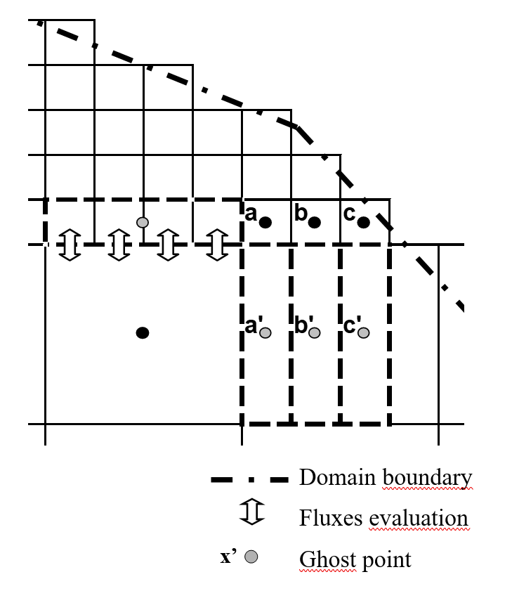
Fig. 1. Border between two adjacent blocks on a Cartesian multiblock grid – Ghost points for the reconstruction of the variables

Appropriate flux computation has always been a challenging issue in computational fluid dynamics. The fluxes \(\bf{f}\) and \(\bf{g}\) are computed by a Flux Vector Splitting (FVS) method, where the upwinding direction of each term of the fluxes is simply dictated by the sign of the flow velocity reconstructed at the cells interfaces. It can be formally expressed as:

\[\begin{split}\bf{f}^{+} = \left( {\begin{array}{*{20}{c}} {hu}\\ {h{u^2}}\\ {huv} \end{array}} \right)\end{split}\]

\[\begin{split}\bf{f}^{-} = \left( {\begin{array}{*{20}{c}}0\\{{{g{h^2}} \mathord{\left/{\vphantom {{g{h^2}} 2}} \right.\kern 1pt} 2}}\\0\end{array}} \right)\end{split}\]

\[\begin{split}\bf{g}^{+} = \left( {\begin{array}{*{20}{c}}{hv}\\{huv}\\{h{v^2}}\end{array}} \right)\end{split}\]

\[\begin{split}\bf{g}^{-} = \left( {\begin{array}{*{20}{c}}0\\0\\{{{g{h^2}} \mathord{\left/{\vphantom {{g{h^2}} 2}} \right.\kern 1pt} 2}}\end{array}} \right)\end{split}\]

where the exponents \(+\) and \(-\) refer to, respectively, an upstream and a downstream evaluation of the corresponding terms. A Von Neumann stability analysis has shown that this FVS ensures a stable spatial discretization of the terms \({\frac{\partial {\bf{f}}} {\partial x}}\) and \({\frac{\partial {\bf{g}}} {\partial y}}\) in Eq. (1) (Archambeau, 2006). Due to their diffusive character, the fluxes \({{\bf{f}}_{\rm{d}}}\) and \({{\bf{g}}_{\rm{d}}}\) can be determined by means of a centred scheme.

Besides low computation costs, this FVS has the advantages of being completely Froude independent and of facilitating the adequacy of discretization of the bottom slope term (Dewals et al., 2006; Dewals et al., 2008a, Archambeau, 2006).

Topography gradients

The discretization of the topography gradients is always a challenging task when setting up a numerical flow solver based on the SWE. The bed slope appears as a source term in the momentum equations. As a driving force of the flow, it has however to be discretized carefully, in particular regarding the treatment of the advective terms leading to the water movement, such as pressure and momentum.

The first step to assess topography gradients discretization is to analyse the situation of still water on an irregular bottom. In this case, momentum equations simplify and there are only two remaining terms: the advective term of hydrostatic pressure variation and the topography gradient. For example, regarding x-axis equation

(11)\[\frac{g}{2}\frac{{\partial {h^2}}}{{\partial x}} = - gh\frac{{\partial {z_b}}}{{\partial x}}\]

The hydrostatic pressure gradient has to be exactly counterbalanced by the bottom slope term. Analytically, the equation can be written as

(12)\[gh\frac{{\partial Z}}{{\partial x}} = 0\]

with \(Z\) the free surface elevation. In case of water at rest, the free surface gradient is equal to zero and thus the free surface is horizontal.

In this case, assuming the bottom elevation and the water height are reconstructed coherently at the finite volume sides and their gradients are identically evaluated (Fig. 2), Eq. (12) can be written as

(13)\[\frac{g}{2}\frac{{\partial {h^2}}}{{\partial x}} = gh\frac{{\partial h}}{{\partial x}}\]

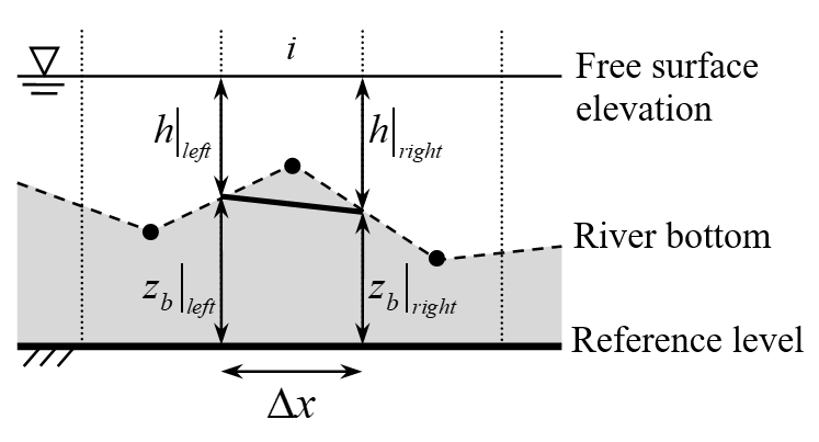
Fig. 2. Correspondence between the gradients of bottom elevation and water depth for water at rest

The space discretization has to provide equivalent conservative and non conservative forms of the pressure gradient. According to the FVS characteristics, a suitable treatment of the topography gradient source term of Eq. 6 is thus a downstream discretization of the bottom slope and a mean evaluation of the corresponding water depths (Erpicum, 2006). For a mesh \(i\) and considering a constant reconstruction of the variables, the bottom slope discretization writes:

(14)\[{\left. { - gh\frac{{\partial {z_b}}}{{\partial x}}} \right|_i} \to - g\frac{{\left( {\left. h \right|_{i + 1}^{} + \left. h \right|_i^{}} \right)}}{2}\frac{{\partial \left( {{{\left. {z_b^{}} \right|}_{i + 1}} - {{\left. {z_b^{}} \right|}_i}} \right)}}{{\partial x}}\]

where subscript \(i + 1\) refers to the downstream mesh along x-axis.

This approach fulfils the numerical compatibility conditions defined by Nujic (1995) regarding the stability of water at rest. The final formulation is the same as the one proposed by Soares (2000) or Audusse (2004).

The formulation is suited to be used in both 1- and 2D models, along x- and y- axis. Its very light expression benefits directly from the simplicity of the original spatial discretization scheme.

Nevertheless, the formulation of Eq. (18) constitutes only a first step towards an adequate form of the topography gradient as it is not entirely suited regarding water in movement over an irregular bed. The effect of kinetic terms is not taken into account and, consequently, poor evaluation of the flow energy evolution can occur when modeling flow, even stationary, over an irregular topography (Erpicum, 2006, Bruwier, 2016).

Time discretization

Since the model is applied to compute (highly) unsteady and/or steady-state solutions, the time integration is performed by means of an explicit Runge-Kutta scheme at various number of time steps.

• 1-step (Euler explicit) first order accurate

• 2-step second order accurate – used for transient computations.

• 3-step first order accurate – providing adequate dissipation in time is valuable for steady-state.

For stability reasons, the time step is constrained by the Courant-Friedrichs-Levy condition based on gravity waves. The time step is thus computed as:

\[\Delta t = \min \left( {\frac{{{\rm{NC \kern 2pt min}}\left( {\Delta x,\Delta y} \right)}}{{\sqrt {{u^2} + {v^2}} + \sqrt {gh} }}} \right)\]

where NC is the Courant number prescribed by the user. The stable value is depending on the Runge-Kutta algorithm used and the local hydrodynamics, but is lower than 1.

A semi-implicit treatment of the bottom friction term is used, without requiring additional computational costs.

Slight changes in the Runge-Kutta algorithm coefficients allow modifying its dissipation properties and make it suitable for accurate transient computations.

Boundary conditions (external or internal)

For each application, the value of the specific discharge can be prescribed as an inflow boundary condition. The transverse specific discharge is usually set to zero at the inflow even if a different value can be used if necessary. In case of supercritical flow, a water elevation can be provided as additional inflow boundary condition.

The inflow boundary conditions can be replaced by infiltration/exfiltration zones. In this case, certain cells are identified in the infiltration array, and the solver computes source terms (mass and momentum) based on the infiltration/exfiltration rate. Multiple infiltration/exfiltration zones can be defined for each model. It is possible to link some of these zones and compute the rate from Bernoulli’s equation based on the local head difference at each time step.

The outflow boundary condition may be a water surface elevation, a Froude number or no specific condition if the outflow is supercritical.

At solid walls, the component of the specific discharge normal to the wall is set to zero.

Topography data

Since 2000, high resolution, high accuracy topographic datasets have become increasingly available for inundation modelling in a number of countries. In Belgium, a data collection programme using airborne laser altimetry (LIDAR) has generated high quality topographic data covering the floodplains of most rivers in the southern part of the country (2002), the whole Region (2013-2014, 2021-2022) and more recently a combined data including bathymetry using green Lidar.

Wolf is very well suited to handle these high resolution datasets.

Methodology for systematic inundation mapping

Following a Regional Government decision in 2003, the solver WOLF2D, has been chosen to be used to compute a part of the official inundation hazard maps on 800 km of the main rivers of the Walloon Region in Belgium. This work has been performed in the scope of flood risk management, insurance of this risk, critical areas identification and climate change effects mitigation policy.

A 4-step modelling procedure has been elaborated and applied systematically for each river reach:

1. Elaboration from laser altimetry and sonar data (or cross sections) of the complete DEM (main riverbed and floodplains) with a grid resolution of 1 m by 1 m,

2. Validation and enhancement of the DEM by a field survey and the integration of additional geometric characteristics,

3. Flow modelling of past flood events with the purpose of calibrating and validating the roughness parameters,

4. Computation of the inundation maps for constant statistical flood discharge values (25-, 50- and 100-year return period and more if necessary).

Depending on the river width, steps 2 to 4 are conducted with a grid spacing varying between 1 m and 5 m, with a typical value of 2 m.

Now, we can deal with native 50 cm resolution data on quite large area using GPU computing.

The use of constant discharges to assess the consequences of flooding is justified by the morphology of the rivers studied. Indeed, as detailed by de Wit et al. (2007), the Meuse basin covers an area of about 33,000 km², including parts of France, Luxembourg, Belgium, Germany and the Netherlands. It can be subdivided into three major geological zones, referred to as “Lotharingian Meuse” (southern part), “Ardennes Meuse” (central part) and the Dutch and Flemish lowlands (northern part).

While the southern and northern parts are characterized by wide floodplains where flood waves are significantly attenuated, in the central part of the Meuse basin, between Charleville-Mézières and Liège, the Meuse is captured in the Ardennes massif, characterized by narrow steep valleys, where flood waves are hardly attenuated.

For instance, for typical floods occurring on the river Ourthe, it has been verified that the volume of water stored in the inundated floodplains along a 10 km-long reach remains lower than one percent of the total amount of water brought by the flood wave.

Therefore, the steady-state assumption has been considered as valid for simulating floodplain inundation along most rivers of the Ardennes Massif.

However, the model natively computes flow in transient mode, including reaching a steady state. It is therefore possible to calculate any flood hydrograph (natural or artificial, like dike breaching or dam break).

Fortran code

WOLF2D is coded in Fortran and compiled as an executable. The code is parallelized using OpenMP.

The code is available on request.

Synthèse des fonctionnalités (Fortran)

• Schéma de discrétisation en espace : volumes finis

• Méthode de reconstruction des inconnues : constante ou linéaire par maille

• Lois de frottement : Manning/Strickler, Barr-Bathurst, Colebrook-White, Bazin, Haaland, Hazen-Williams

• Discrétisation spatiale : grillage cartésien, potentiellement multi-blocs

• Discrétisation temporelle : Euler, RK21, RK22, RK31, RK32, RK42

• Précision de calcul : virgule flottante double précision (64 bits)

• Conditions aux limites : débits spécifiques, hauteurs d’eau, altitude de surface libre, Froude, conditions internes (type barrage, pont en charge…)

• Zones d’infiltration/exfiltration : nombre illimité, interpolation linéaire

• Mise à jour de la topographie en cours de calcul : possible

Note

Le pas de temps est calculé automatiquement par le code en fonction de la vitesse de propagation des ondes de gravité et de la vitesse de l’écoulement. Il est possible de spécifier un nombre de Courant cible pour ajuster la stabilité du calcul.

Ordre de grandeur :

• vitesse de calcul : 1.5 millions de mailles / seconde en RK31 sur un processeur Intel i7

• pas de temps : de 0.01 à 0.1 seconde pour des écoulements de type crue sur maillage de 1 mètre

Mise en place d’une modélisation multi-blocs

Il est possible de créer une modélisation multi-blocs via l’interface graphique ou via script (plus flexible).

Afin de créer une telle simulation 2D, les étapes principales sont :

• créer une instance prev_sim2D en lui passant en argument le chemin d’accès complet et le nom générique de la simulation

• définir un contour vectoriel/polygone délimitant la zone de travail

• (optionnel) définir une “grille magnétique” servant d’accroche des vertices des polygones (permet de s’aligner entre différentes modélisations par ex.)

• définir la résolution spatiale du maillage sur lequel les données (topo, frottrement, inconnues…) seront fournies initialement

• définir des contours/polygones des blocs et leur résolution spatiale respective

• appeler le mailleur (appel au code Fortran)

• créer les matrices obligatoires et les remplir avec les valeurs souhaitées (via script(s) ou GUI)

• créer les bords potentiels pour les conditons aux limites (.sux, .suy)

• imposer les conditions aux limites nécessaires (info : rien == imperméable)

• paramétrer le problème

• exécuter le calcul

• traiter les résultats

Un notebook d’exemple 1 est disponible pour illustrer ces étapes. Ce Notebook est assez complet pour expliquer la mise en place, le paramétrage, l’imposition des conditions aux limites, l’exécution et l’affichage des résultats.

Un notebook plus court est également disponible pour une mise en place plus rapide de la même simulation.

Note

Vous disposez déjà d’une modélisation opérationnelle et vous souhaitez en créer une copie en modifiant les paramètres ? Un notebook d’exemple 2 est disponible pour illustrer ces étapes.

Vous disposez déjà d’une modélisation opérationnelle et vous souhaitez la convertir en modélisation GPU ? Un notebook d’exemple 3 est disponible pour illustrer ces étapes.

Afin de créer une modélisation depuis l’interface graphique, il faut ouvrir le code wolf2d ou wolf et cliquer sur “File / Create/Open Multiblock model”.

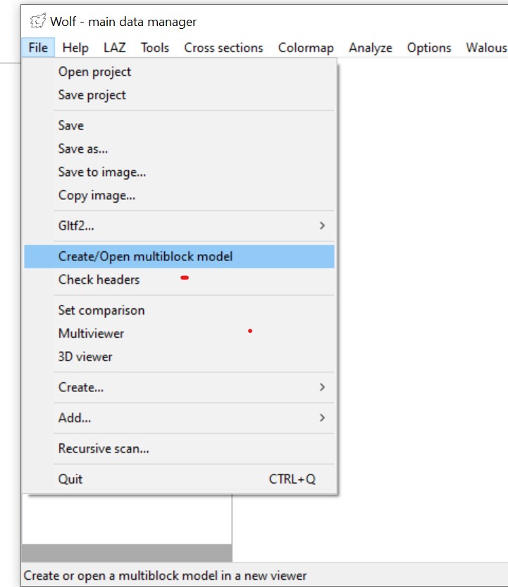
Une nouvele fenêtre s’ouvre alors, permettant de choisir le répertoire de stockage de la simulation. Après avoir validé, un viewer spécifique pour le modèle est créé.

Une fenêtre de paramétrage s’ouvre alors, permettant de définir la géométrie et les paramètres de la simulation.

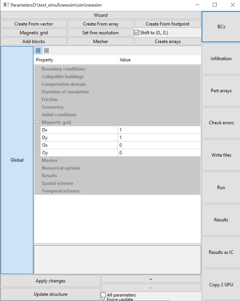
Le premier bouton est un Wizard décrivant succinctement les étapes nécessaires à la création d’une simulation multi-blocs.

Il est possible de définir la géométrie :

• sur base du vecteur/polygone actif

• sur base de la matrice active (contour extérieur == masque de la matrice)

• sur base d’une emprise définie par les coordonnées de l’origine, le nombre de mailles selon chaque direction et la résolution spatiale

Il est ensuite possible de :

• définir une grille magnétique pour faciliter l’alignement des vertices des polygones entre simulations

• définir la résolution fine du maillage

• de forcer la translation des vertices des polygones à la coordonnée (0., 0.) - souvant nécessaire car les opérations de maillage s’effectuent en Float32 côté Fortran et les coordonnées Lambert sont mal adaptées pour conserver la pleine précision de calcul

• d’ajouter des blocs et de les paramétrer (voir zone centrale de la fenêtre)

• d’appeler le mailleur

• de créer des matrices vides (le nombre et le type de matrices dépend du choix du modèle - par ex. pas de .kbin et .epsbin sans modèle de turbulence)

La colonne de droite est dédiée aux opérations de simulations :

• imposer les conditions aux limites

• gérer l’infiltration

• (optionnel) définir les matrices sur base d’une liste de fihciers

• vérifier d’éventuelles erreurs de paramétrage avant calcul

• écrire les paramètres sur Disque

• lancer le calcul (via wolfcli.exe)

• afficher les résultats

• convertir les résultats en conditions initiales

• convertir le modèle en version GPU (voir aussi le Jupyter Notebook dédié)

Pour le paramétrage, il existe des paramètres :

• globaux

• de blocs

Il est possible de cliquer sur autant de boutons de blocs que souhaité. Le premier bouton est considéré comme la référence.

Si les autres blocs possèdent le même paramétrage, leur bouton sera vert. Si des paramètres diffèrent, le bouton sera rouge. Une déselection de la référence transfère la référence au deuxième.

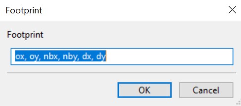
La liste des paramètres qui diffèrent est affichée dans la case textuelle en bas de fenêtre

Note

Pensez à aggrendir la fenêtre verticalement si elle n’est pas visible

Un clic sur le bouton “Global” désactivera tous les blocs et activera les paramètres globaux.

En cas de modification simultanée via scipt et GUI, un bouton “Update structure” permet de relire les paramètres en mémoire et remplir les widgets graphiques.

Warning

Si quelque chose ne se passe pas comme prévu, pensez à regarder la fenêtre de logging.

Un problème persiste ? Contactez le support technique.

Note

Envie d’en savoir plus sur le code, explorez les classes suivantes:

• Wolf2DModel

• prev_sim2D

GPU code

WOLFGPU est une version GPU du code WOLF2D. Il est écrit en Python et OpenGL 4.6.

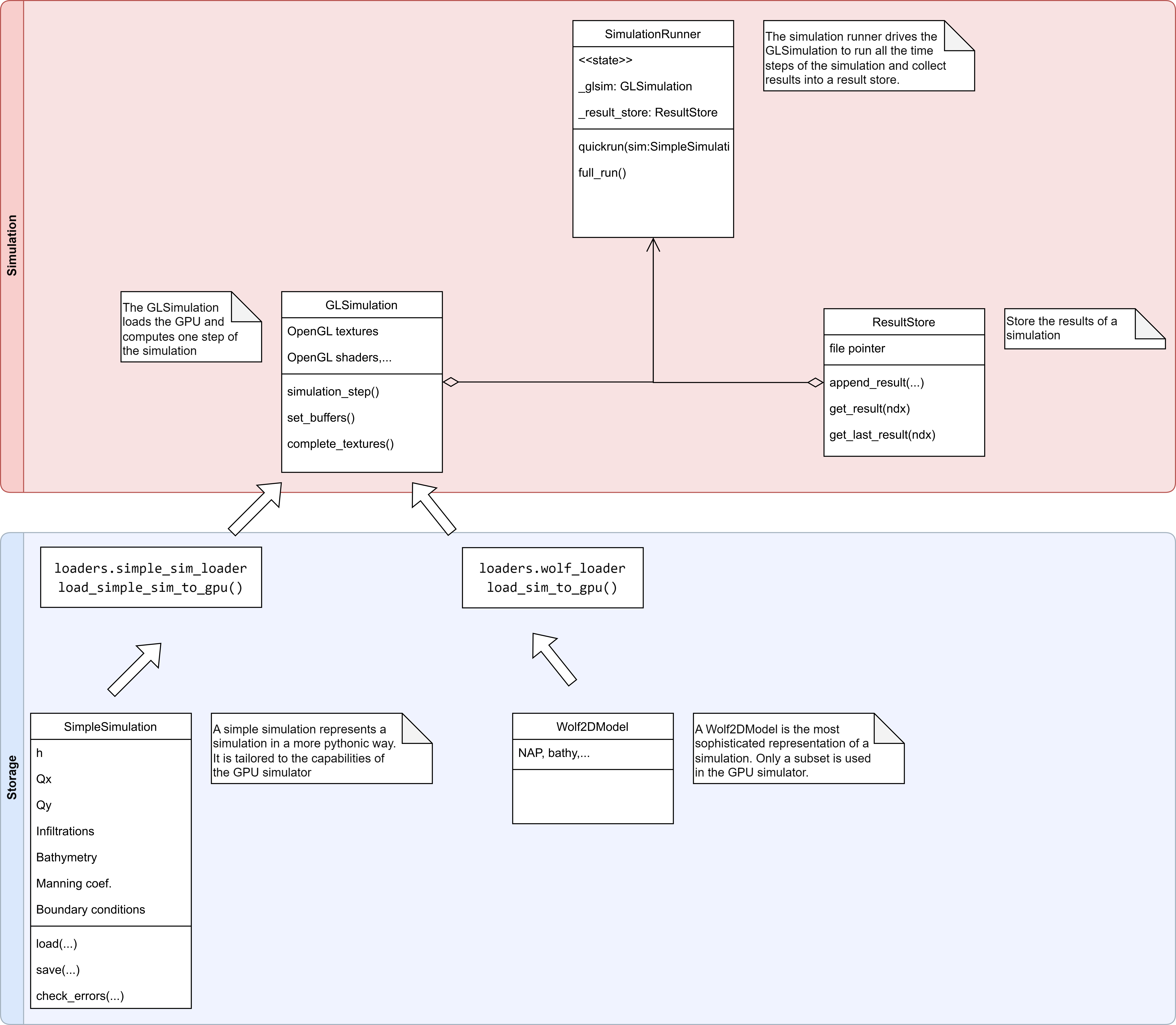
Architecture

Le code GPU peut s’appuyer sur deux structures d’entrée différentes:

• une modélisation WOLF2D compatible avec le Fortran, ce qui permet de réutiliser des modélisations existantes

• une structure plus simple, appelée “SimpleSimulation”, qui permet de le mettre en place facilement par l’API

Une instance GLSimulation est créée à partir de l’une de ces structures. Cette instance est ensuite utilisée par le SimulationRunner pour piloter la simulation.

Les résultats sont affichés en temps réel dans une fenêtre OpenGL.

Le reporting des résultats est géré par le ResultStore qui assure l’écriture et la relecture des inconnues de calcul mais également des métadonnées associées (pas de temps, temps total simulé…).

Note

Les résultats sont actuellement stockés sous la forme de matrices Numpy au format Compressed Sparse Row.

Ceci peut cependant évoluer sans préavis. La rétro-compatibilité sera assurée via le ResultStore uniquement.

Une autre classe Python gère l’affichage des résultats dans la fenêtre graphique du viewer. Cette classe peut potentiellement mettre les résultats en cache afin d’accélérer l’analyse sur plusieurs pas de temps.

Synthèse des fonctionnalités (GPU)

• Schéma de discrétisation en espace : volumes finis

• Méthode de reconstruction des inconnues : constante par maille

• Lois de frottement : Manning/Strickler

• Discrétisation spatiale : grillage cartésien, taille de maille unique

• Discrétisation temporelle : RK21, RK22

• Précision de calcul : virgule flottante simple précision (32 bits)

• Conditions aux limites : débits spécifiques, hauteurs d’eau, altitude de surface libre, Froude

• Zones d’infiltration/exfiltration : nombre illimité, interpolation linéaire ou constant par palier

• Mise à jour de la topographie en cours de calcul : oui

Note

Le pas de temps est calculé automatiquement par le code en fonction de la vitesse de propagation des ondes de gravité et de la vitesse de l’écoulement. Il est possible de spécifier un nombre de Courant cible pour ajuster la stabilité du calcul.

Ordre de grandeur :

• vitesse de calcul : 500 millions de mailles / seconde en RK22 sur un processeur Intel i9 et carte RTX3090

• pas de temps : de 0.01 à 0.1 seconde pour des écoulements de type crue sur maillage de 1 mètre

Benchmarking

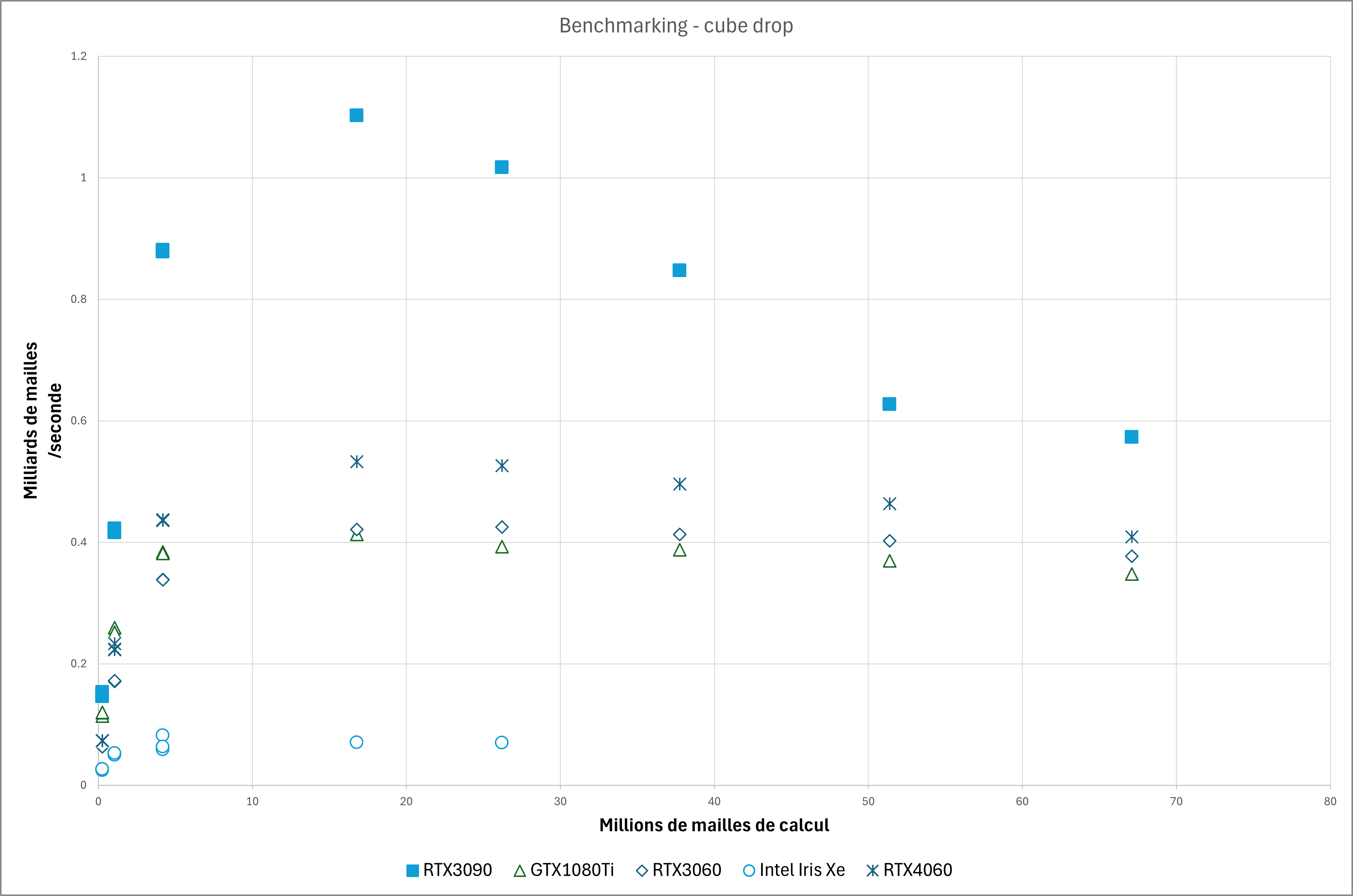
Une option de benchmarking est disponible pour tester les performances du code sur différentes cartes graphiques.

Le benchmarking consiste à exécuter le code sur des grilles carrées de tailles:

• 512 x 512

• 1024 x 01024

• 2048 x 2048

• 4096 x 4096

• 5120 x 5120

• 6144 x 6144

• 7168 x 7168

• 8192 x 8192

Le problème est un bac aux parois impermaéables avec une hauteur d’eau initiale nulle, sauf sur une colonne centrale.

Les résultats sont enregistrés dans un fichier CSV.

Note

Pour information, la machine de test la plus puissante est équipée du matériel suivant:

• processeur Intel i9-12900KF (16 coeurs)

• carte mère Asus Prime Z690-P

• 128 Go DDR5 4800

• Disque SSD Samsung 980 Pro 1To + HDD WD 4To

• Windows 11 Pro 64 bits

Cinq cartes graphiques ont été testées sus Windows10/11:

• Nvidia RTX3090 (PC ci-dessus)

• Nvidia RTX3060

• Nvidia RTX4060

• Nvidia GTX1080Ti

• Intel Iris Xe (Portable Surface Pro 8)

Les caractéristiques des cartes graphiques sont les suivantes:

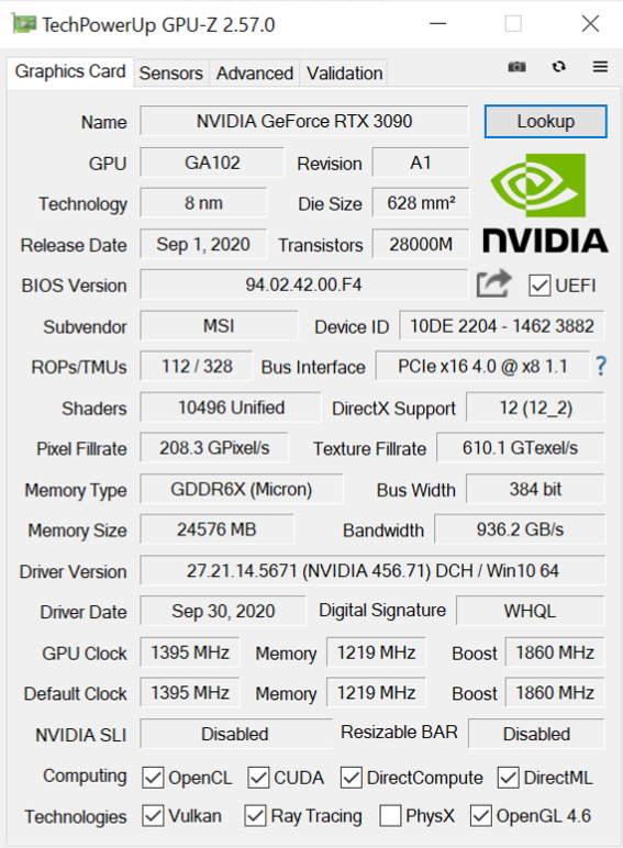
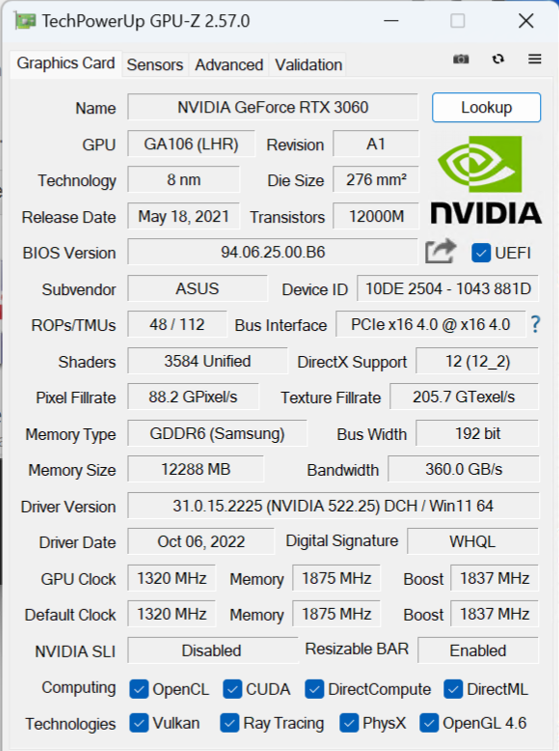
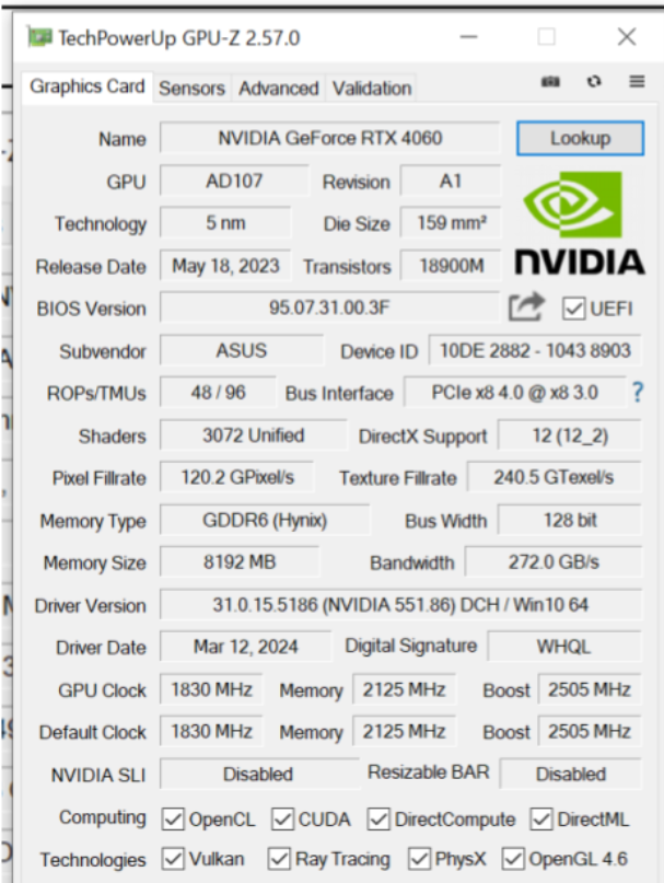
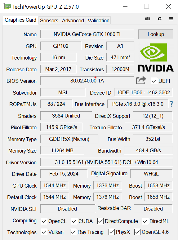
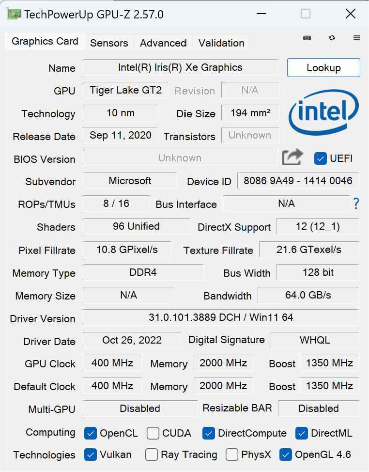
Le graphique suivant montre les performances des différentes cartes sur base du nombre de noeuds calculés par seconde en fonction de la taille du problème.

Note

Il est possible d’obtenir un code plus rapide en exploitant certains paramètres liés notamment à la gestion de l’assèchement (-dry-up-loops) ou au tiling (-tile-size ; -no-tiles-packing). Il est toutefois du ressort du modélisateur de faire ces choix en connaissance de cause.

Des travaux sont encore en cours afin de poursuivre l’optimisation du code (utilisation mémoire et vitesse pure).

Exécution de l’application

L’application peut être exécutée en utilisant la commande suivante :

wolfgpu

Il est également possible de lancer le code via un appel python:

python -m wolfgpu.cli

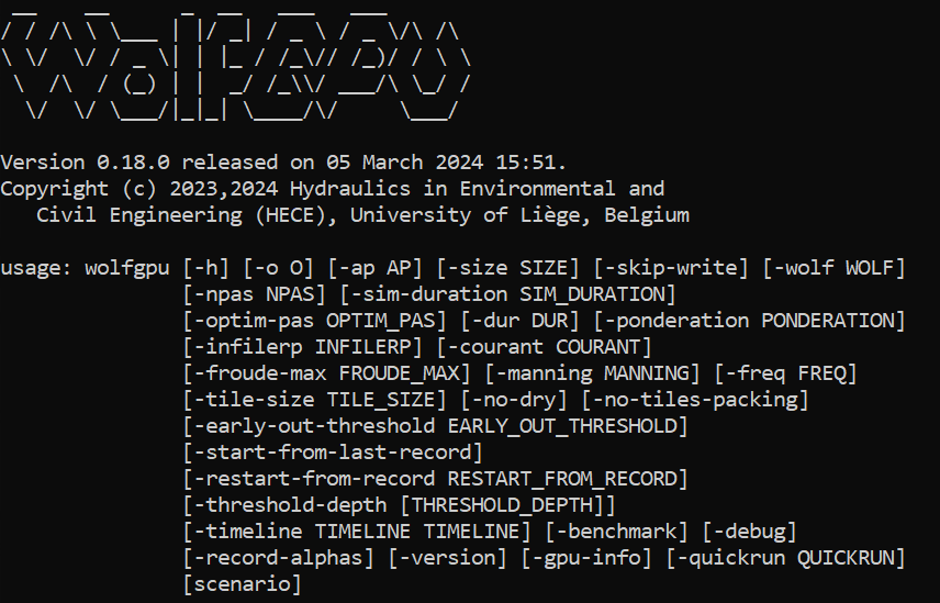
Il est possible de spécifier des options pour l’application. Pour obtenir la liste des options disponibles, il est possible d’utiliser la commande suivante :

wolfgpu --help

Scenario intégré :

Exécution du scenario “cube drop” disponible avec le code

Note

Ceci est peut-être anodin pour certains mais il est bon de remarquer que le code reste totalement symétrique sur toute la durée de l’exécution.

Premier modèle

Un modèle simple sur base d’un Jupyter Notebook est disponible.

Ce fichier illustre les étapes pour préparer les données, lancer le code de calcul et accéder aux résultats par 2 moyens différents.

Exécution de l’application sur une machine équipée de plusieurs cartes graphiques

A l’heure actuelle, l’application wolfgpu n’exploite qu’une seule carte graphique. Seules les cartes NVidia (GTX ou supérieure) et une carte intégrée Intel ont été testées.

Warning

Toute carte avec des capacités OpenGL 4.6 devrait pouvoir exécuter le code.

Toutefois, la compilation du code est effectuée sur la carte et par le driver du constructeur. Il n’est donc pas possible de garantir le bon fonctionnement de l’application sur toutes les cartes graphiques du marché.

De même, l’implémentation des opérateurs mathématiques dépend également du constructeur de la carte graphique. Aucune garantie de reproductibilité totale, c’est-à-dire une stricte comparaison binaire des résultats pour plusieurs exécutions succesives ou sur des machines différentes, n’est donc possible sans test approfondi du matériel.

Si la machine est équipée de plusieurs cartes graphiques, il est normalement possible de spécifier la carte à utiliser en utilisant le panneau de contrôle (par exemple “NVidia Control Panel”) et en particularisant la carte à utiliser pour le rendu OpenGL.

Cette option est normalement disponible pour un exécutable en particulier.

Note

Afin de le rendre applicable sur nos PC, il a été nécessaire de dupliquer l’exécutable python.exe, par exemple python1.exe, python2.exe…

Après avoir adapté le paramètre “Processeur graphique de rendu OpenGL” dans le panneau de contrôle NVidia, il est possible d’exécuter l’application avec la commande python1.exe -m wolfgpu.cli.

Dupliquer le script wolfgpu.exe ne semble pas fonctionner sans pour autant en avoir déterminé la raison exacte.

Bibiography

• Audusse, E., 2004. Modélisation hyperbolique et analyse numérique pour les écoulements en eaux peu profondes. Ph.D. Thesis, Laboratoire Jacques-Louis Lions, Université Paris VI – Pierre et Marie Curie, France.

• de Wit, M., Peeters, H., Gastaud, P., Dewil, P., Maeghe, K., Baumgart, J., 2007. Floods in the Meuse basin: event description and an international view on ongoing measures. International Journal of River Basin Management, 5(4): 279-292

• Nujic, M., 1995. Efficient implementation of non-oscillatory schemes for the computation of free-surface flows. Journal of Hydraulic Research, 33(1): 101-111

• Soares Frazão, S., 2000. Dam-break induced flows in complex topographies – Theoretical, numerical and experimental approaches. Ph.D. Thesis, Université Catholique de Louvain, Belgium.

• HECE