2D cell indices
In this notebook, we show the differences that exist between coordinates and indices on a grid.
Moreover, we show the difference between the Wolf array conventions (which are born out of the Fortran language) and the numpy array conventions.
Our code base uses the two simultaneously and being comfortable with them will help you a lot.
Note that a WolfArray is built on top of a numpy array but with a major difference: a WolfArray numbers its indices as (x, y) whereas in numpy, the indices are (y,x). That difference comes from the long history of Wolf arrays which begins in the Fortran world.
[ ]:
import matplotlib.pyplot as plt
import numpy
from wolfhece.assets.mesh import Mesh2D, header_wolf
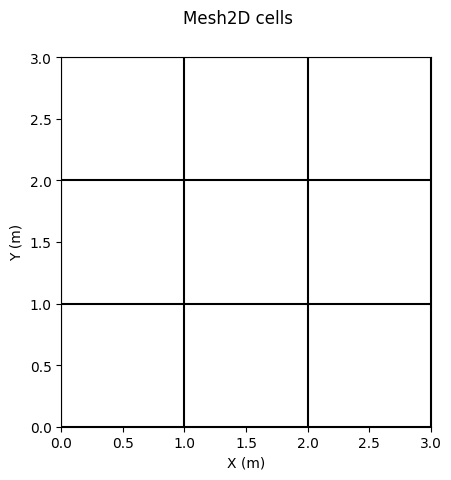
Creation of a 2D grid
number of cells along X = 3
number of cells along Y = 3
[2]:
h = header_wolf()
h.set_origin(0., 0.)     # origx, origy
h.set_resolution(1., 1.) # dx, dy
h.shape = (3,3)          # nbx, nby
[ ]:
grid = Mesh2D(h)
Viewing the Grid as Coordinates/Georeferenced item
In this perspective, the X-Y coordinate system follows a right-handed (dextrorsum) orientation:
The X-axis extends horizontally from left to right and is measured in meters.
The Y-axis extends vertically from bottom to top and is measured in meters.
[ ]:
fig, ax = grid.plot_cells() # plot cells
fig.suptitle('Mesh2D cells')
Text(0.5, 0.98, 'Mesh2D cells')
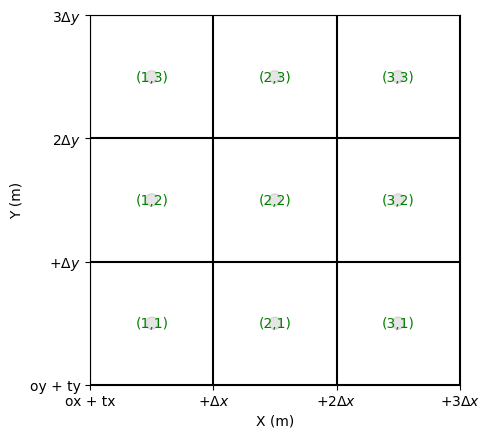
Cell/Mesh Numbering
The indices of the meshes follow this convention:
Rows evolve along the X-axis.
Columns evolve along the Y-axis.
Thus, the index \([i, j]\) corresponds to the position:
\([origx + (i - 0.5) dx, \, origy + (j - 0.5) dy]\)
where:
\(origx\) is the x-coordinate of the origin (in local or global coordinates, adjusted by \(translx\) if applicable).
\(origy\) is the y-coordinate of the origin (in local or global coordinates, adjusted by \(transly\) if applicable).
\(dx\) is the resolution along the X-axis.
\(dy\) is the resolution along the Y-axis.
[5]:
fig, ax = grid.plot_cells()
grid.set_ticks_as_dxdy(ax)
grid.plot_circle_at_centers(ax, radius = .05, alpha = 0.1) # plot circle at centers
grid.plot_indices_at_centers(ax=ax, color='green', fontsize = 10) # plot indices at centers
[5]:
(<Figure size 640x480 with 1 Axes>, <Axes: xlabel='X (m)', ylabel='Y (m)'>)
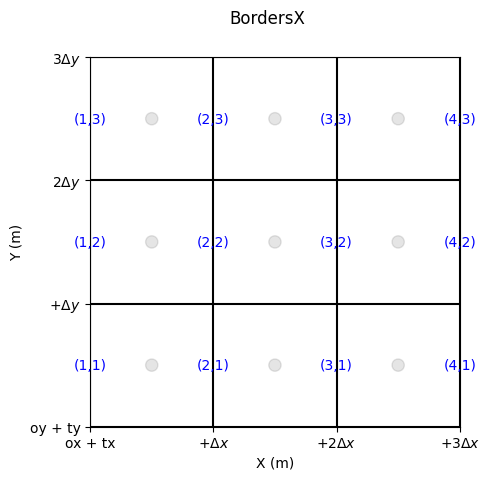
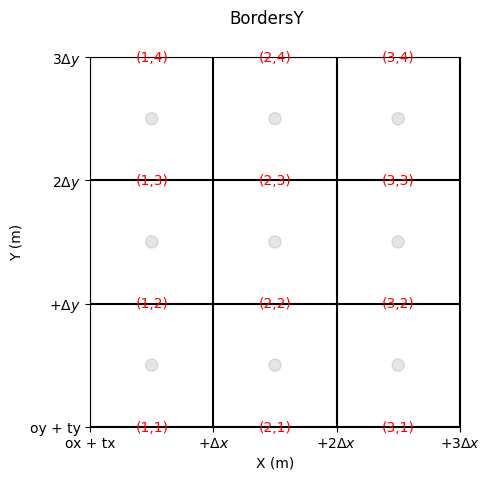
Edge Numbering
Edges are also indexed.
We distinguish:
the bordersX, i.e., those whose normal flux is aligned with X (the edge itself is aligned with Y)
the bordersY, i.e., those whose normal flux is aligned with Y (the edge itself is aligned with X)
[6]:
fig, ax = grid.plot_cells() # plot nodes
grid.set_ticks_as_dxdy(ax)
grid.plot_circle_at_centers(ax, radius = .05, alpha = 0.1) # plot circle at nodes
grid.plot_indices_at_bordersX(ax=ax, color='blue', fontsize = 10) # plot indices at bordersX
fig.suptitle('BordersX')
[6]:
Text(0.5, 0.98, 'BordersX')
[7]:
fig, ax = grid.plot_cells() # plot nodes
grid.set_ticks_as_dxdy(ax)
grid.plot_circle_at_centers(ax, radius = .05, alpha = 0.1) # plot circle at nodes
grid.plot_indices_at_bordersY(ax=ax, color='red', fontsize = 10) # plot indices at bordersX
fig.suptitle('BordersY')
[7]:
Text(0.5, 0.98, 'BordersY')
Shape
a matrice storing cells values has a shape (nbx, nby)
a matrice storing bordersX values has a shape (nbx+1, nby)
a matrice storing bordersY values has a shape (nbx, nby+1)
[8]:
print('Cells matrice - shape : ',grid.zeros().shape)
print('BordersX matrice - shape : ',grid.zeros_bordersX().shape)
print('BordersY matrice - shape : ',grid.zeros_bordersY().shape)
Cells matrice - shape :  (3, 3)
BordersX matrice - shape :  (4, 3)
BordersY matrice - shape :  (3, 4)
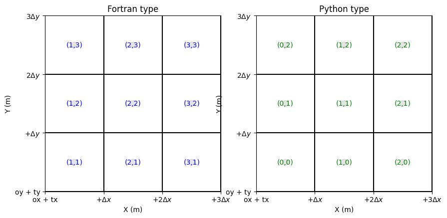
Fortran/Python Numbering
Fortran is 1-based.
Python is 0-based.
In routines, you have a parameter named ‘aswolf’. If it is True, the Fortran convention is applied. Generally, “True” is the default value but read the routine’s docstring if necessary.
Boundary condition indices must be provided using the Fortran-type (1-based).
[14]:
fig, ax = plt.subplots(1,2, figsize=(10,5)) # plot nodes

grid.plot_cells(ax=ax[0]) # plot cells
grid.set_ticks_as_dxdy(ax[0])
grid.plot_circle_at_centers(ax[0], radius = .05, alpha = 0.1) # plot circle at nodes
grid.plot_indices_at_centers(ax=ax[0], Fortran_type=True, color='blue', fontsize = 10) # plot indices at bordersX
ax[0].set_title('Fortran type')

grid.plot_cells(ax=ax[1]) # plot cells
grid.set_ticks_as_dxdy(ax[1])
grid.plot_circle_at_centers(ax[1], radius = .05, alpha = 0.1) # plot circle at nodes
grid.plot_indices_at_centers(ax=ax[1], Fortran_type=False, color='green', fontsize = 10) # plot indices at bordersX
ax[1].set_title('Python type')
[14]:
Text(0.5, 1.0, 'Python type')
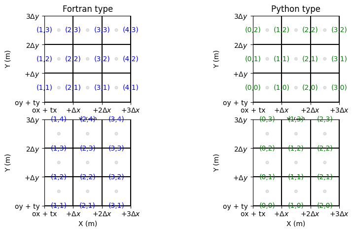
[13]:
fig, ax = plt.subplots(2,2, figsize=(10,5)) # plot nodes

grid.plot_cells(ax=ax[0,0]) # plot cells
grid.set_ticks_as_dxdy(ax[0,0])
grid.plot_circle_at_centers(ax[0,0], radius = .05, alpha = 0.1) # plot circle at nodes
grid.plot_indices_at_bordersX(ax=ax[0,0], Fortran_type=True, color='blue', fontsize = 10) # plot indices at bordersX
ax[0,0].set_title('Fortran type')

grid.plot_cells(ax=ax[0,1]) # plot cells
grid.set_ticks_as_dxdy(ax[0,1])
grid.plot_circle_at_centers(ax[0,1], radius = .05, alpha = 0.1) # plot circle at nodes
grid.plot_indices_at_bordersX(ax=ax[0,1], Fortran_type=False, color='green', fontsize = 10) # plot indices at bordersX
ax[0,1].set_title('Python type')

grid.plot_cells(ax=ax[1,0]) # plot cells
grid.set_ticks_as_dxdy(ax[1,0])
grid.plot_circle_at_centers(ax[1,0], radius = .05, alpha = 0.1) # plot circle at nodes
grid.plot_indices_at_bordersY(ax=ax[1,0], Fortran_type=True, color='blue', fontsize = 10) # plot indices at bordersX

grid.plot_cells(ax=ax[1,1]) # plot cells
grid.set_ticks_as_dxdy(ax[1,1])
grid.plot_circle_at_centers(ax[1,1], radius = .05, alpha = 0.1) # plot circle at nodes
grid.plot_indices_at_bordersY(ax=ax[1,1], Fortran_type=False, color='green', fontsize = 10) # plot indices at bordersX
[13]:
(<Figure size 1000x500 with 4 Axes>, <Axes: xlabel='X (m)', ylabel='Y (m)'>)
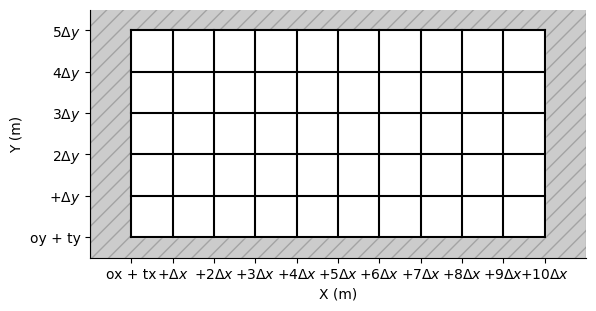
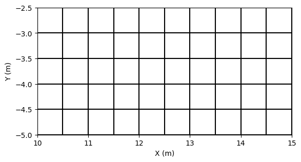
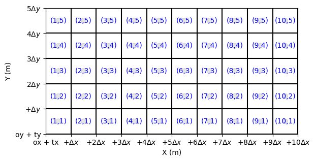
Exploring a More Complex Grid Configuration
In this section, we apply the previously discussed concepts to a grid where the number of cells along the X and Y axes differ. This demonstrates how the grid structure adapts to varying resolutions and dimensions.
[9]:
h2 = header_wolf()
h2.set_origin(10., -5.)     # origx, origy
h2.set_resolution(0.5, 0.5) # dx, dy
h2.shape = (10,5)          # nbx, nby
[10]:
grid2 = Mesh2D(h2)
fig, ax = grid2.plot_cells() # plot cells
[11]:
fig, ax = grid2.plot_cells() # plot nodes
grid2.set_ticks_as_dxdy(ax)
grid2.plot_circle_at_centers(ax, radius = .05, alpha = 0.1) # plot circle at nodes
grid2.plot_indices_at_centers(ax=ax, color='blue', fontsize = 10) # plot indices at bordersX
[11]:
(<Figure size 640x480 with 1 Axes>, <Axes: xlabel='X (m)', ylabel='Y (m)'>)
[12]:
fig, ax = grid2.plot_outside_domain() # plot outside domain
grid2.plot_cells(ax) # plot nodes
grid2.set_ticks_as_dxdy(ax)
grid2.scale_axes(ax, .1) # scale axes by 2.0
[12]:
(<Figure size 640x480 with 1 Axes>, <Axes: xlabel='X (m)', ylabel='Y (m)'>)